Partial-Fourier imaging at High Resolutions

This blog post discusses the resolution loss when applying partial-Fourier imaging in GE-EPI in the presence of strong T2*-decay.

I found that that when I was aiming for high-resolutions, it is beneficial to refrain from the application of partial Fourier (PF) imaging as much as possible. For the long readout durations at high-resolutions and the fast T2/T2*-decay at high field strengths results in even stronger blurring of partial-Fourier.

Example 1 of the blurring with and without partial Fourier imaging

Example 2 of the blurring with and without partial Fourier imaging

The magnitude point spread function is an uninterpretable measure of spatial resolution

Many of the MRI education books suggest that a center-out T2* weighting like in SE-EPI and with partial Fourier imaging would theoretically result in a sharper point spread  function (PSF) (Jesmanowicz et al., MRM, 1998; Hyde et al., MRM, 2001; Hetzer et al., MRM, 2011). This really goes against my experience of real-live data (examples above) and hence, I tried to implement my own simulations below. Based on those simulations, I conclude that the magnitude PSF may be sharper for partial Fourier imaging, however it is not an adequate measure of the spatial resolution. The effective spatial resolution is better without partial Fourier imaging.

I tired to investigate the effect of T₂^*-attenuation during the EPI readout theoretically in two ways:

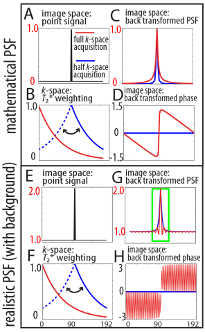
1. conventional magnitude PSF estimation, where only one voxel is assumed to differ from zero (Delta function in panel A). The corresponding signal distribution in k-space is then weighted with the T₂^*-decay for full k-space GE-EPI and half (PF) GE-EPI (panel B), respectively (dotted: mirrored in GE-EPI). The back-transformation into image space provides the PSF (panel C) and the phase distribution (panel D) of the EPI signal.
2. Additionally, I did the same estimation for a more realistic situation resembling edges/contrast: namely, that only one voxel has a signal different from a finite background signal (panel E). This example is introduced to show the different effect of the complex PSF compared to the magnitude PSF. The same T₂^*-decay was introduced as described above (panel F) and the corresponding T₂^*-blurring in image space was calculated (panel G/H).

In addition to these theoretical simulations, I tried to investigate the  T₂^*-blurring in-vivo. Two different readout strategies were used to estimate the different T₂^*-blurring: full k-space acquisition (readout window = 110 ms) and half k-space acquisition (readout window = 60 ms) with the same TE. In order to correct for phase inhomogeneities in the half k-space acquisition, 8% of the k-space lines were acquired symmetrically, across the center of k-space.

Conventional estimation of the PSF associated with T₂^*-blurring (one voxel ≠ 0; Fig. A) and full k-space GE-EPI gives a larger FWHM compared to PF half k-space EPI PSF (Fig. C). Note that due to the step in the phase distribution (Fig. D), the real and the imaginary part of the PSF have a narrower FWHM in full k-space GE-EPI than in PF half k-space EPI (Figs. I/J). For the adapted way of estimating T₂^*-blurring (Fig. E), the magnitude PSF of full k-space GE-EPI has a narrower FWHM than that of PF half k-space EPI (Fig. G). This is a result of positive and negative interference of signal from adjacent voxels depending on their phase.

The experimental data confirm that full k-space acquisition appears to give better spatial specificity in the phase encoding direction than PF half k-space acquisition (Figs. M/N). Intracortical anatomical layers are blurred in the phase-encoding direction (white arrows), but not in the read direction (black arrows) for the PF half k-space GE-EPI (Fig. M). The discriminability of the intra-cortical layer-dependent signal peaks (Figs. O and P) confirms this (green arrows). Correspondingly, during a finger tapping task, the functional profiles delineated layer-dependent responses with higher effective resolution for the full k-space GE-EPI scheme compared to the case where T₂^*-attenuation is symmetric in k-space (Figs. Q/R).

Conclusion

The conventional usage of the width of the magnitude PSF to estimate T₂^*-blurring can be misleading. In order to take into account that MRI produces complex signals, which can add up constructively or destructively, the PSF must be considered in the complex domain (Figs. I-L). I show here that full k-space GE-EPI acquisition has a higher effective resolution than partial-Fourier k-space GE-EPI.

My intuitive explanation for the blurring with PF

It is well described that outer k-space lines represent the high spatial frequencies and the k-space lines close to the k-space center represent the smooth spatial frequencies. Hence, when partial Fourier is applied, the outer k-space lines are under represented and the image will look blurrier. Without partial Fourier imaging, one side of k-space is has a relatively large signal and the other side of k-space has a relatively low signal due to T2*-decay. Hence, the suppression of the later-acquired outer k-space lines is accounted for by the large signal of the firstly acquired outer k-space lines. The result is a sharper signal of a out-center-out k-space acquisition trajectory compared to partial Fourier imaging, even though the FWHM of the magnitude point spread function is larger.

The reconstruction method matters

At high resolutions, the EPI protocol is often limited by too long TEs. Hence, it is not easily possible to simply refrain from the application of PF imaging. In a good fraction of my experiments, I also need to apply it to some extent. In those cases, when the application of PF imaging is not avoidable, special care should be taken to reconstruct the partly acquired k-space with the appropriate reconstruction algorithm.

Example of the effect of different reconstruction methods. POCS can recover some of the high-resolution information that is lost for conventional zero-filling.

How to change the reconstruction in the sequence code:

Zero-filling

There are a couple of algorithms already implemented from SIEMENS. The default in fMRI sequences is the algorithm of “Zero filling”. You can find this in the sequence code as “None”:
pSeqExpo->setPCAlgorithm          (SEQ::PC_ALGORITHM_NONE);
This option has the worst blurring. However, because of the blurring, it also has the highest SNR. I would assume that this is the reason, why it is set as default.

Margosian

You can also choose the algorithm “MARGOSIAN”. In the sequence code this can be set as follows:
pSeqExpo->setPCAlgorithm (SEQ::PC_ALGORITHM_MARGOSIAN);
With MARGOSIAN, the missing k-space lines are not just zero-filled. Instead, they are filled with the complex conjugate of the symmetric acquired k-space lines. This algorithm results in less blurring. However, I find it very unstable and sensitive to phase-inconsistencies and B0-inhomogeneities. I also found it to result in additional void artifacts. The resulting tSNR is very low.

Submatrix

You can also choose the algorithm “SUBMATRIX”. In the sequence code this can be set as follows:
pSeqExpo->setPCAlgorithm (SEQ::PC_ALGORITHM_SUBMATRIX);
I don’t really understand what it does. But the final results are not much better than with Zero-filling.

POCS

Another option is POCS (projection onto convex sets). In my opinion, this is the best option. In the sequence code it look as follows:
pSeqExpo->setPCAlgorithm          (SEQ::PC_ALGORITHM_POCS_PE);
or for 3D readouts:
pSeqExpo->setPCAlgorithm          (SEQ::PC_ALGORITHM_POCS_3D);
The working principle it very similar to MAGROSIAN. In my understanding, the only difference is that it accounts for B0-inhomogeneities by allowing an asymmetric k-space and filing in the missing k-space lines iteratively.
This method is quite stable against phase inconsistencies.

However, the default number of POCS iterations is 2! This is a very low number and should be increased. In most cases, the POCS algorithm converges to a stable solution in 2-4 iterations. I always set it to 8. This increases the reconstruction time by a few milliseconds and is completely worth it.
I don’t know how to change the number of POCS iterations in the sequence code. However, I know how it can be set in xbuilder after the registration of the participant as described in the figures.

This slideshow requires JavaScript.

How to change the reconstruction if you don’t have the sequence code:

There is a corresponding parameter in /MedCom/config/Ice/IceConfig.evp under:

MEAS -> sKSpace -> ucPOCS

If it is not set in the sequence, already you might be able to switch on the POCS parameters here. In my experience, most sequences have this parameter already set explicitly. Thus, changing the ucPOCS in the IceConfig file has not effect on the reconstruction.

Alternatively, the POCS reconstruction can be set via the xml file in the retro-recon.

PC_ALGORITHM_NONE 0
PC_ALGORITHM_MARGOSIAN ?
PC_ALGORITHM_3D_MARGOSIAN ?
PC_ALGORITHM_SUBMATRIX ?
PC_ALGORITHM_3D_SUBMATRIX ?
PC_ALGORITHM_POCS_PE ?
PC_ALGORITHM_POCS_RO 256
PC_ALGORITHM_POCS_PE 512
PC_ALGORITHM_POCS_3D 1024
PC_ALGORITHM_POCS_RO_PE 765
PC_ALGORITHM_POCS_RO_3D 1280
PC_ALGORITHM_POCS_PE_3D 1536
PC_ALGORITHM_POCS 1792

The number on the right refers to the value that you would need to fill in for “PCAlgorythm”.

Partial Fourier related signal voids

In the Figure above, it can be seen that POCS and MAGROSIAN reconstructions result in darker stripes in the image magnitude compared to zerro filling. I think that parts of these black PF-voids are coming from the fact that in unfortunate cases the signal in one side of k-space is opposite to the other side of k-space. Thus, both sides of k-space cancel each other out (opposite k-space positions have the opposite phase and point in opposite directions, canceling each other out). For full-k-space sampling this canceling is not present because the opposite magnetization direction is can be simply stored in the image phase, without affecting the magnitude. Similarly in zero-filling, when the image phase is zero, all the magnetization is assumed to have the same direction anyway and no cancellation is present.
For MAGROSIAN and POCS, the phase is not zero but regularized. Thus, the cancellation effect can happen.

I think the cancellation effect can be avoided, if we would apply the PF reconstruction only after the coil combination. The coils introduce so many phase differences and they are quite different across elements. After combining the elements the phase is much more homogeneous and POCS can be applied much more effectively.

Another source of Partial Fourier related signal voids can come from the fact that -compared to full k-space acquisition- partial Fourier acquisition have a shorter readout. This means that voxels with a large within-voxel gradient along the phase-encoding direction results in a shift of the effective echo time. In extreme cases the k-space center for such voxels is pushed outside EPI k-space sampling window. This would mean that the k-space center would be captured in lines that are not captured for Partial Fourier acquisition. Thus, in contrast to full k-space acquisition, this signal is lost. Since this signal is not acquired for PF imaging to begin with, it cannot be recovered with any reconstruction method.

Amount of partial-Fourier

Of course, it the amount PF-induced blurring depends on the amount of omitted k-space lines. In my experience, partial Fourier imaging with a factor of 7/8 in combination with POCS reconstruction can recover most of the high-resolution information.

Comparison of zero-filling and POCS filling

Comparison of PF in GE-EPI and SE-EPI

In when PF is applied in GE-EPI, the outer k-space lines are suppressed. This is similar in spin echo EPI. The only differente is that in SE-EPI the T2-decay results in an asymmetric k-space weighing onto of the additional symmetric T2* weighing. My simulations below suggest that the resulting blurring in SE-EPI is not as bad as the application of PF.

Alternative measured of blurriness

Since the magnitude point-spread function is an elusive measure of the blurriness of an image, it tried to look at alternative measures. An Alternative measure of the effective resolution is the distance that two signal sources of the voxel size need to have to be separable as two individual objects. As the animations below show, with the application of PF, the point sources need to be further apart to be separable as two individual objects compared to full k-space imaging.

Partial Fourier blurring without strong T2*

When zero filling is applied, the application of partial Fourier imaging can result in image blurring even with fast readouts (with minimal T2*-decay). This effect has is discussed in great detail from practiCal fMRI in this blog post. In this post, he also discusses other advantages and disadvantages of PF imaging, including the increased SNR and amplified void artifacts.

Partial Fourier and the blooming effect of large veins in BOLD (from Joseph Vu)

The void artifacts (esp. in the case of zero filling) likely also exacerbates large vein bias since large veins tend to have strong susceptibility gradients as well. This bias will appear in the individual T2* weighted images as “blooming artifacts” around the large veins , but it also has the capability of enhancing BOLD CNR disproportionately in these large vessels – which is bad if the goal is mesoscale fMRI. So definitely, minimizing the use of PF or turning on POCS is a good idea for mesoscale fMRI.

Common misconceptions with respect to Partial Fourier

• The application of partial Fourier does not affect the amount of EPI distortions. The amount of EPI-distortions is solely determined by the echo-spacing (how fast neighboring k-space lines are acquired). When the echo time is reduced by parallel imaging acceleration or by changes in the bandwidth, an echo time reductions comes along with reduced distortions. This is not the case for echo time reductions due to the application of Partial Fourier.
• For a given echo-train (e.g. with Partial Fourier), changing the TE does not affect the PSF. For example, when the echo time is increased to be longer than the minimum echo time, the Partial Fourier blurring and the distortions will be the same. The only thing that changes is T2* contrast.
• Many users tend to be afraid of going out to longer TEs when in fact BOLD CNR is optimal and quite robust at surprisingly long TEs as shown by van de Zwaag et al 2009. Especially given effective T2* should increase as voxel sizes decrease, users should be encouraged to pilot protocols with various TEs and partial Fourier factors to see what works best for them. This is perhaps particularly relevant in the context of TE dependent, layer dependent BOLD sensitivities (Koopmans et al 2011). (Comment from Joseph Vu).

Quotes from the experts:

• Using partial-Fourier is just like taking drugs; You know it’s bad for you and that you shouldn’t use it. But when you sit at the scanner you suddenly get the urge to use it. And think: I will use it just the once, I promise. Jon Polimeni, April 26th 2017, Hawaii.
• With slow gradients and fast decay, partial-Fourier is the only way to have enough signal. Its better to have a blurry image than no image at all. David Feinberg, Februar 26th 2018, Berkeley.
• Its completely expected that when you omit the acquisition of outer k-space lines that represent the high spatial frequencies the effective resolution will be decreased. I never trusted the magnitude PSF anyway. Larry Wald, Februar 13th 2014, Leipzig.

Further reading

• The basics of Partial Fourier imaging are explained on
  • mriquestions.com and
  • MR-Tip.com and
  • CBS-harvard.
• Both the application of partial-Fourier sampling and the application of parallel imaging increase the acquisition speed and reduce the echo time. Hence, it is often advised to only use one of the two. practiCal fMRI has an excellent blog post about the comparison of partial Fourier and GRAPPA here.
• We had an abstract about the inadequate interpretation of the magnitude point-spread-function at ISMRM in 2015 (see poster here).
• Derek Jones’ Diffusion MRI book also has a good section on the interaction of Partial Fourier and Motion, which is another can of worms! The book can be found here. (Thanks to Joseph Vu for the tip.)

Acknowledgments:

I learned all about partial Fourier imaging in discussion with Ben Poser, Valentin Kemper, Peter Koopmans, and Franz Patzig. I want to thank them for their input. I also want to thank Joseph Vu for his comments (below) that shaped a revision of a some sections.