The paper that explains the sequence and its parameter regime is can be found here: https://www.ncbi.nlm.nih.gov/pubmed/23963641. The sequence diagram looks something like this:

There are different readouts implemented so far:

• single-shot EPI
• multi-echo
• SMS-EPI
• SMS-Multi-echo (with the WIP recon from MHG)
• 3D-CAIPI-EPI

They are all implemented in VB17-UHF.

Inversion timings

The Inversion time “TI2” (as visible in the sequence editor) refers to the time between the center of the inversion pulse and the center of the first excitation pulse of the first readout module.
The other inversion time parameters TI1 and TI1s are not used and are remnants from earlier versions of the sequence. Just leave them at the very short default value.
The time difference of the two readout modules is adjusted with the sequence card “TR” parameter. It is adjusted in a way that all images are equally spaced across time. There is no option to independently adjust the second readout pulse from the first one.

The sequence is set up in a way that the delay period between BOLD and VASO is the same as the delay period between VASO and BOLD. This is theoretically not necessary for the contrast generation of VASO. Its just the easiest way how it is implemented in the sequence code.

Calculation of the blood nulling time.

Conventional steady-state VASO approaches use the equation TI = T1 * (ln (1+chi) – ln(1+chi*exp(-TR/T1))). With chi being the inversion efficiency [0:1]. Since SS-SI VASO assumes that the blood magnetization is inverted only once, I use the equation TI = T1 * ln(1+chi).
The inversion efficiency chi is affected by two things: (A) the phase skip of the inversion pulse, (B) T2 relaxation during the adiabatic inversion. The (B) part is negligibly small and is often ignored. If you want to include everything in one equations it reads:
TI = T1_blood * ln(1+cos(phase_skip)*exp(-(0.5*pulse_duration)/(T2_blood))). Usually, I assume a blood T1 = 2100 ms, blood T2 = 45 ms. In M1 I use a phase skip of 30deg. In V1, I use a phase skip of 0deg (with Nova inversion coils).
In V1, I would end up with desired TIs of 2100 * ln(1+cos(0)*exp(-(0.5*10)/(45))) = 1342 ms.
In M1, I would end up with desired TIs of 2100 * ln(1+cos(30)*exp(-(0.5*10)/(45))) = 1200 ms.

Adjustment of the TI parameter in the protocol editor of the sequence.

Note, that the above discussion refer to effective “TI”, the blood nulling time. The desired time of the blood signal acquisition. The “TI” in the sequence editor, however, only refers to the first excitation pulse, not the center time point of the imaging volume. Hence, when the readout block takes about 600ms. The “TI” in the sequence editor must be correspondingly earlier.

In M1, for a readout duration of 600 ms, I would adjust the “TI” in the sequence editor to 900 ms. In V1, it would be 1050 ms.

Inversion pulse parameters

The adiabatic inversion pulse is calculated in real time and can be adjusted within the sequence editor. Optimal parameters are duration 10 ms, BWDTH 300%, amplitude between 90 and 110 %.
Those are also the default values and have been adjusted based on a series of pilot experiments (http://pubman.mpdl.mpg.de/pubman/item/escidoc:1752750:3/component/escidoc:1752749/VASO_Thesis_Huber.pdf Figures 6.2, 6.3, 6.15, 6.18, 6.22).
The performance of the pulse should be stable -independent of the amplitude. Only if the adiabaticity threshold is undershot, the inversion efficiency might suffer. The minimum B1+ needed for good inversion efficiency is 7-10 muT. With the Nova coil, this is achieved with amplitudes of > 90% (Ref ampl 220V). There is almost no disadvantage of going to high amplitudes. It is only limited by SAR. Common inversion efficiency parameters are in the range of 90% (in phantoms).
If you change the bandwidth, it will affect the sharpness of the pulse (Fig. 6.3). Values below 300 % (6.355 kHz) make the pulse less sharp. Higher values reduce the adiabaticity and make the pulse more susceptible to B1+ inhomogeneities.

The thickness parameter is only used, when the Phase-skip is switched off. For a head transmit coil, it is advised to always use a phase skip. E.g. in visual cortex for flickering checkerboard use, Phase-skip = 1. In Motor cortex for Phase skip use 30 deg. When doing breath hold , phase skips of 60deg might ne necessary (with loss in SNR).

While the original VASO paper shows gradients during the inversion pulse, I have come to the conclusion that at 7T it is best to have the slab-thickness as large as possible. Hence, from the sequence code perspective, the inversion is a global inversion. In reality it is an “slab-selective” inversion, where the slab thickness is determined by the size of the transmit coil. Only at 3T with a body transmit coil the gradients become important again.

Inflow effects

Since the advent of VASO in 2003, inflow effects and corresponding CBF-contamination have been a serious concern in functional VASO experiments. Manus Donahue investigated inflow effects for conventional VASO variants with steady-state blood in his paper. He found out that in conventional VASO, inflow effects result in a negative VASO signal change. Hence, they amplify the negative CBV-weighted VASO signal change.

This is different for SS-SI VASO. In SS-SI VASO, inflow effects have the opposite effect. There, CBF contaminations are caused by inflow of blood that has not been inverted at all. I.e. blood that was outside the inversion coverage below the circle of willis during the adiabatic inversion and has flown into the imaging slice until the signal is acquired. This ‘fresh’ blood has a large (equilibrium) magnetization. When the vessel is engaged in the functional task and changes its diameter and flow velocity, the arterial arrival time becomes shorter during activation. As a result, the amount of the large arterial equilibrium magnetization increases even more and results in a CBF-dependent signal increase during activation, which counteracts the negative CBV-contrast in VASO. 

The occurrence of such inflow effects is highly dependent on multiple experimental aspects, including: transmit coil coverage, inversion pulse efficiency, and functional task. Since the arterial arrival time is highly variable across brain areas, inflow effects are differently pronounced across ROIs.

While local activation tasks (e.g. flickering checkerboards and/or finger tapping) do not change the arterial arrival times of the large vessels and result in minimal inflow effects, global tasks (e.g. breathhold, CO2-breating) are expected to be much more susceptible to inflow effects.

Identification of inflow effects

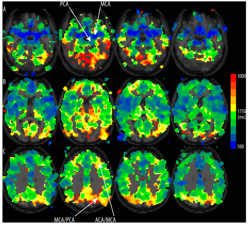
1. Looking out for bright voxels. In an IR sequence like the VASO sequence, large vessels are refilled for short TIs and are filled with equilibrium magnetization after 200-1000 ms. Hence, they look like very short T1 compartments. Thus, also in VASO, inflow of fresh blood results in easily visible isolated bright voxels (Van De Moortele et al., 2009). Here, we can utilize this effect and quantify the occurrence of inflow-driven voxels as a measure of how much VASO is contaminated by inflow. The very large arteries, that are detectable with this trick do not necessarily pose a problem in functional VASO, because they are not functionally engaged in the functional task. That is because these vessels are similarly refilled with fresh blood during rest and during tapping, so they do not mask the tapping-induced signal changes.
2. Looking out for inverse VASO contrast: Inflowing blood has a large magnetization. If the vessel is engaged in the functional task, the arterial arrival time becomes shorter and the amount of this large arterial magnetization increases even more during activation. This results in a CBF-dependent raw signal increase. So, Inflow effects are clearly visible as an inverse VASO contrast. In functional VASO data, this effect is clearly visible above the cortical surface.

Inflow effect visible as bright voxels in T1-weighted EPI. Data kindly provided by Tanja Dadakova and Alex Beckett from Berkley

Inflow effect visible as a inverse VASO contrast in the same voxels. Data kindly provided by Tanja Dadakova and Alex Beckett from Berkley

Dealing with inflow effects

1. Excluding voxels from further analysis. I found that in the majority of cases, inflow effects are very local and easily detectible. Since inflow-voxels exhibit an inverse VASO contrast, they are already inherently excluded from statistical activation maps.
2. Reducing the blood-nulling time (TI). This can be achieved by reducing the inversion efficiency of the adiabatic inversion pulse. This approach has been described in section 4.3.1 (Page 123ff) of the PhD thesis here.

Tipps for maximal SNR

• FLASH grappa is better than LIN-PAR (FLEET) is better than PAR-LIN is better than single-shot is better than segmented
• make the TR as short as possible. in conventional VASO is reduced the SNR. in SS-SI-VASO in maximizes the SNR.

• Since, its an inversion-recovery sequence the Ernst-angle can be bigger than 90deg! A flip angle in the range of 120deg has the best SNR. A flip angle in the range of 60deg has the nicest T1-weighting.
• Making a longer TI, increases SNR
• Keep TE as short as possible.
• Do the BOLD correction with the interleaved division instead of the T2* fitting to hypothetical TE=0ms.
• With the high-res 3D-EPI protocol after version 121, Flip angle schemes of 4 or 26 are pretty good. The PSF in slice direction is not perfect, however.

Confusing UI artefacts in protocol editor

• All three labeling schemes are doing the same thing: SS-SI VASO. Previous versions of the sequence had also options of Q2TIPS in the UI. These options were not functional and used SS-SI VASO either way.
• The saturation band in the GUI can be ignored. It is also an artifact from ASL. The pulses are not played out and the saturation band in the patient localizer have absolutely no meaning. I just don’t know how to program the GUI, so they still appear in the viewer, even though the corresponding pulses are excluded. The inversion pulse is automatically adjusted to the imaging volume (without showing it in the GUI)

Tips for adjusting the protocol

Order of adjusting the parameters

1. Number of slices
2. Matrix-size
3. Acceleration in slice direction
4. Acceleration in phase direction (including the GRAPPA reference scheme: FLASH)
5. Bandwidth
6. TE
7. TR

Issues in adjusting the parameters

• NEVER EVER TRUST THE SOVLVE HANDLER.
  • In the worst cases is freezes Syngo,
  • If you trust the PNS calculation in one direction it can shut down the gradient amplifier -> Reboot
  • When the solve handler pop-up shows up always choose “undo”, never choose “calculate”.
• Do not go into the red area of parameters. It will open the solve handler saying e.g. that the  TR will be adapted. In both cases (clicking “ok” or clicking “undo”) will gray out the entire protocol editor. -> insert sequence from scratch.
• In latest 3D-EPI versions, the FA is not given in degrees, it rather refers to the #th column in a matrix.

Tested Sequence Protocols

https://github.com/layerfMRI/Sequence_Github

I learned that different sites can achieve different TEs?!? Not clear why. Maybe the gradients are calibrated differently, allowing different effective slew-rates?

TI timing in SMS-VASO

Of course, the TI calculation is dependent on the slice order (Ascending/Descending/Interleaved) in the field “Series:

I think the default is “Descending”, so I will try to explain this scheme in more detail here.

The necessary parameters are:

• #Slices = the total number of slices in the volume
• #SMS = SMS factor, the number of simultaneously acquires slices.
• #SlicesInBlock = number of slices in one block = #slices/#SMS
• TI = inversion time
• TRmin = shortest possible TR allowed by sequence protocol.
• AcquisitionDuration = time that is used to acquire all slices = TRmin – TI
• DeltaTI = time between two consecutive RF-excitation pulses = AcquisitionDuration/#SlicesInBlock

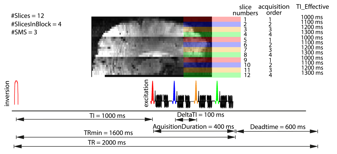
For an descending acquisition order, the top slice is acquired first. And in SMS it is simultaneously acquired with slice 1 x #SlicesInBlock, 2 x #SlicesInBlock, 3 x #SlicesInBlock ….

So, based on the number of slices, the SMS-factor and the Series, the acquisition order can be inferred.

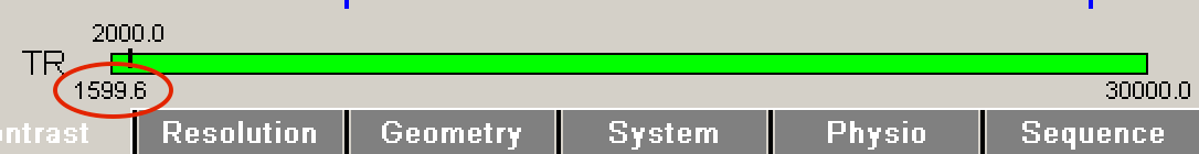
The more complicated part is to find out DeltaTI. Option 1 is that it is given out from the  sequence code with  mySeqLoop.getlKernelScanTime() (in micro seconds). If you don’t have the sequence code it can be estimated by calculating the difference TRmin – TI and dividing it by the SMS factor. TRmin can be seen in the protocol editor at the scanner:

Number of TRs (repetitions) in SS-SI VASO 

The VASO sequence is build on the sequence code of ASL, thus it’s reconstruction pipeline is expecting pairs of images.  And the different versions of VASO may behave weirdly.

In the multi-echo 2D-EPI sequence, the task card only allows even number of TRs and they are all reconstructed. Hence, the reconstructed data will also contain even number of TRs. However, there is the special case when GRAPPA is switched off. In this case and additional image is acquires. The very first image is then a non-steady-state M0-equilibrium image and the reconstructed time-series has odd number of TRs.

In the SMS-VASO sequence, the number of receptions adjusted in the protocol editor should be even and then all time points will be reconstructed properly.

In the newer 3D-EPI sequences, the BOLD task cards allows to adjust even and odd number of TRs. However, when an even number is used, the last time point can get lost in the reconstruction.

Just to be on the safe side, I always add additional three measurements at the end of every scan. This helps in the BOLD correction and gives extra leeway in case the last image is lost. It is to note, however, that the fMRI task does not end before the three additional images are acquired. Otherwise the participant thinks the scan is completed and will move during the last TRs.

Value of TR

In most of the VASO versions (VASO_1 – VASO_151) the TR refers to the number of images and not the number of image pairs. For example, a 80s scan with an TR of 2s (in the protocol editor), you would end up with 20 VASO images and 20 BOLD images. This follows the TR naming convention of the ASL literature and the COBIDAS reporting standard.

In the VASO sequence versions VASO_1-VASO_122, BOLD and VASO images are acquired symmetrically. This means the interleaved acquired BOLD and VASO images have the same TR.

In later VASO versions (starting from version VASO_123 – VASO_151+), the BOLD dead time was removed. This means that TR of all the odd and all the even images are different. E.g. for DMN protocols of visual protocols, the VASO TR will be in the range of 2.7-2.8s, while the BOLD TR is in the range of 2s. Thus, for both together, it takes about TR_eff =4.8-5s. Note that in those sequences, the protocol editor will only display the longer VASO TR.

This means that the effective TR = 4.8s is about 60% longer than the early VASO studies in the motor cortex with TR = 3s. This comes from the fact that FOVs of the new protocols with 26x162x216-matrizes have more than 100 times more voxels compared to the early motor protocols with 32x32x7 matrix sizes. And it takes some time acquire those extra voxels.

In the even later VE sequence versions RENLAY_1 – RENLAY_15, the TR naming convention is different. In those sequences, the TR refers to the pair TR (the effective TR in the figure above).

Please note that in some sequence versions, there might be a minimal mismatch of the TR that you type in to the protocol editor and the TR that the scanner eventually uses. This is due to multiple reasons. E.g. in the SMS-VASO sequences, the FAT-saturation time estimation is done per slice. However, since less pulses are uses more time is saved than expected. So, the TR inaccuracies are dependent on the number of slices and the acceleration factor. Thus, I advise everyone to consider these small sequence bugs in the presentation of the task and the functional analyses. E.g. I advise to present block designed stimuli based on trigger counting, not based on absolute time. And I advise to look at the logfile to make sure that the TR is as expected.

Flip angles in the 3D-EPI sequence

T1 relaxation during readout

In inversion-recovery sequences such as for VASO, T1-relaxation processes can affect the image contrast while a volume is being acquired. In the 2D-SMS sequence, the individual slice-groups are acquired consecutively. This means that adjacent slices can have different T1-weightings. For short TIs ( < tissue T1), this can result in different signal intensity across the brain volume imaged (see figure above). This is different for 3D-EPI. The fact that in 3D-EPI, the entire brain volume has the same effective TI can be advantageous with respect to these TI-inconsistencies across slices. The different effective T1-weighting and the correspondingly different signal across k-space segments in 3D-EPI, however, can result in inhomogeneous signal distribution across k-space. This can result in image blurring along the second phase encoding direction. To account for this and preserve the available MR signal across k-space segments, our 3D-EPI-VASO sequence uses variable flip angle modulations. The concept of using variable flip angles to account for  T1-decay during a multi-shot 3D-readout is adapted from Gai et al. 2011.

Note, however, that this approach of using variable flip angles in 3D-EPI can only serve as a first order correction to minimize T1-related blurring in the second phase-encoding (segment) direction. There are numerous higher-order effects that can not be corrected for with this approach. For instance, the approach of variable flip angles can be optimized for one T1-compartment, only. In our sequence, the nominal flip angles are adjusted to the T1 of GM (1.8 s). This means that the blurring effect in WM and CSF are only partly accounted for. Hence the point-spread-function is expected to be different across different tissue types. Furthermore, the approach of variable flip angles is limited by the inhomogeneities in RF transmit field at 7 T. Hence, in brain regions with particularly high or low B1+ field strengths, the T1-related blurring effect might be only partially accounted for.

In the sequence code, the exact shape of the variable flip angle distribution is calculated based on the adjusted TR, TI, and delta TI of the protocol in real time.

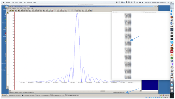
The exact pulse shape used

The excitation pulse is a (non-adiabatic) sinc-like pulse as provided by the scanner manufacture. The pulse shape is shown in the figure below. For the sake of comparison, a sinc shape is overlaid on top of it.  The excitation pulse used appears to be a filtered apodized sinc pulse shape.

Accuracy of the flip angle

On the Siemens platform user interface, flip angles can be specified to integer precision.

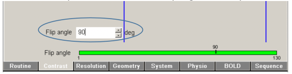
This interface is only used to adjust the final flip angle of the multi-shot readout (90 deg). The preceding pulse flip angles are calculated in real time from the sequence code without this precision limitation.

In the sequence code, the relative differences of the RF pulses can be adjusted to a precision of 6-7 digits.

See the screenshot of the sequence-development environment:

The same precision is used for the global RF scaling:

This of course does not mean that the RF amplifiers used and the resulting B₁⁺ field have the same accuracy. Thus in publication manuscript is is advised to use the term desired nominal flip-angles that the sequence code is adjusted to.

RF-clipping of variable flip angles

When the excitation pulse duration (in the special card) is very short and/or the Bandwidth-time-product (in the special card) is very large, it can easily happen that the RF-peak power is exceeding the maximum value that is allowed by the system (RF amplifiers). The sequence code realizes this and scales the pulse amplitude down, that the peak power is not exceeding the maximum anymore. This does not affect the relative pulse shapes. I.e., the pulse shape will not end up with a flat top. Instead, the entire pulse train is scaled down by the same value. Note, however, that the scaling is done individually for every excitation pulse of every individual k-space segments. Thus, the relative ratio of the excitation pulses of all k-space segments can be affected. E.g. when the last pulse of the excitation pulse train exceeds the maximal value by 20% but the first pulse does not exceed the maximum, only the last pulse is scaled down, making the first and the last pulse more similar.

One easy way to find out if you are in this regime, is that the SAR increases for longer pulse durations.

Flip angle parameter in the protocol editor

The adjustable flip angle in the protocol editor refers to the flip angle of the fist k-space segment. The flip angles of all successive k-space segments is calculated based on GM T1 (1.8s), TR, TI and delta TI of the current protocol. The whole chain of flip angles is written out (with cout) at the MPCU. At the scanner you can look at this out put by starting “telnet mpcu” while the sequence is prepared for a scan.

Sequence versions with version numbers bigger than VASO_114 have additional features for the flip angle field in the protocol editor (in the contrast task card). There are 8 predefined flip angle distributions strategies estimated in real time and stored as a big Flip angle matrix. E.g. when you choose a value of “4” in the field of the flip angle, it does not refer to 4 degrees. Instead, it refers to the 4th column in the flip angle matrix. This allows the operator to have additional degrees of freedom with respect to choosing a sensitivity-specificity compromise.

RF clipping can be beneficial

The figure below shows three potential flip angle distributions, their corresponding PSF and example images.

• The first column refers to the application of the Ernst angle, which is in the range to 18 deg for typical VASO values. This means, however, that at the end of the readout there is a lot of z-magnetization left that could have been harvested to increase the SNR.
• The second column refers to a distribution, where the flip angle increases between segments with a faster rate then what the T1-relaxation can account for. This results in more magnetization been harvested and larger SNRs. However, it also means that the k-space segments have inconsistent weighting, which results in a broader PSF and signal blurring.
• In the third column, an additional cut-off is introduced. The results means that even more z-magnetization is harvested compared to the middle column. Thus it have an even higher SNR than the middle column. With such an asymmetric k-space weighting, however, the PSF becomes complex and has an imaginary part that can result in destructive interference between neighboring k-space segments (see negative side-lobes of the PSF). These side-lobes can partly account for the blurring in the middle column, while maintaining the high SNR.

Based on these considerations it can be beneficial to introduce a bit of RF-clipping

Other T1 compartments.

Since the variable flip angle is adjusted for one T1 compartment only, other T1 compartments (E.g. WM and GW) will have a different point spread function.

Often, this can result in a edge enhancement artifact. as shown below.

This effect can be partly accounted for by applying a corresponding weighting in k-space of retrospectively, with the “-laurencian’ option in the LAYNII program LN_DIRECT_SMOOTH.

File locations of the 3D-EPI sequence for VB17 (for installation)

The 3D-EPI sequence on VB17 uses the 3D-EPI from Benedikt Poser with the respective reconstruction files that need to be stored at specific locations. Here is a list of all of them:

C:/MedCom/bin/IceMosaic2D3D.dll
C:/MedCom/bin/IceMosaic2D3D.dll
C:/MedCom/bin/IceMosaic2D3D.evp
C:/MedCom/bin/IceMultiecho_WIP.dll
C:/MedCom/bin/IceMultiecho_WIP.evp
C:/MedCom/bin/IceNewOnlineTSE.dll
C:/MedCom/bin/IceNewOnlineTSE.evp
C:/MedCom/bin/IceNoiseCorrelation.dll
C:/MedCom/bin/IceNoiseCorrelation.evp
C:/MedCom/bin/IceOptimalGrappa4EPI.dll
C:/MedCom/bin/IceOptimalGrappa4EPI.evp
C:/MedCom//MriCustomer/IceConfigurators/BPIceProgramMultiEcho_WIP.evp
C:/MedCom/MCIR/Med/lib/libIceOptimalGrappa4EPI.so
C:/MedCom/MCIR/Med/lib/libIceMosaic2D3D.so
C:/MedCom/MCIR/Med/lib/libIceMultiecho_WIP.so
C:/MedCom/MCIR/Med/lib/libIceNewOnlineTSE.so
C:/MedCom/MCIR/Med/lib/libIceNoiseCorrelation.so
C:/MedCom//MriCustomer/seq/BP_evaprot_WIP.evp
C:/MedCom//MriCustomer/seq/VASO_124.dll
C:/MedCom//MriCustomer/seq/VASO_124.i86

If you already have some of the files on your system, do not overwrite them. In this case, I would advise to use the ones that you already have.