3rd order shim for layer-fMRI: To get best data quality, avoid certain EPI frequencies.

On Oct 13th 2023, Nicolas Boulant presented an intriguing source of MRI image artifacts at the CMRR high field meeting in Minnesota. He suggested that the 3rd-order shim can result in amplified gradient trajectory imperfections. In low bandwidth FLASH, this can manifest as faint ghosts in the read direction shifted by a few pixels. In EPI, on the other hand, these trajectory errors can result in fuzzy ripples (low spatial frequency ghosts and shadings, not edge ghosts). 

In a recent meta analysis of all openly available layer-fMRI datasets, I had found had that the fuzzy ripples are one of the main limits of high-quality layer-fMRI acquisition (see here) across vendors. So, I was curious whether the 3rd order shim might be partly related to this. In this blog post, I am describing my attempts to reproduce Nicola’s results and investigate the effect of the 3rd order shim on layer-fMRI protocols. I find that disconnecting the 3rd order shim can result in significantly better data quality. However, this finding is only visible for specific echo-spacings, which are either in the ‘forbidden frequencies’ or which have side bands in the forbidden frequencies.

This post does not imply that previous research was conducted sub-optimally. Since, it is common practice to optimize the EPI echo spacing in the piloting stage of each study, the frequencies with these artifacts are usually avoided anyway. Here, we confirm that this is a good practice.

Continue reading “3rd order shim for layer-fMRI: To get best data quality, avoid certain EPI frequencies.”

NORDIC denoising on VASO data

Authors: Lasse Knudsen, Luca Vizioli, Federico De Martino, Lonike Faes, Dan Handwerker, Renzo Huber

This post describes the usage, capabilities and challenges of NORDIC PCA denoising on VASO data. A video presentation of this project can be found here: https://youtu.be/bbGKMTWVrJY.

Continue reading “NORDIC denoising on VASO data”

Equi-voluming: The Anakin Skywalker of layering algorithms

Authors: Renzo Huber and Faruk Gulban

When you want to analyze functional magnetic resonance imaging (fMRI) signals across cortical depths, you need to know which voxel overlaps with which cortical depth. The relative cortical depth of each voxel is calculated based on the geometry of the proximal cortical gray matter boundaries. One of these boundaries is the inner gray matter boundary which often faces the white matter and the other boundary is the outer gray matter boundary which often faces the cerebrospinal fluid. Once the cortical depth of each voxel is calculated based on the cortical gray matter geometry, corresponding layers can be assigned to cortical depths based on several principles.

One of the fundamental principles used for “assigning layers to cortical depths” (aka layering, layerification) is the equi-volume principle. This layering principle was proposed by Bok in 1929, where he tries to subdivide the cortex across little layer-chunks that have the same volume. I.e. gyri and sulci will exhibit any given layer at a different cortical depth, dependent on the cortical folding and volume sizes (see figure below).

With respect to applying equi-volume principle in layer-fMRI, the equi-volume layering has gone through quite a story. A plot with many parallels to Anakin Skywalker.

In this blog, the equi-volume layering approach is evaluated. Furthermore, it is demonstrated how to use it in LAYNII software.

Continue reading “Equi-voluming: The Anakin Skywalker of layering algorithms”

Quality assurance measures for layer-fMRI time series: How to obtain them in LAYNII

Doing layer-fMRI sometimes feels like doing nothing more than noise management. One must have a full grown masochistic personality trait to enjoy working with such messy data. Namely, layer-fMRI time series data suffer from each and every one of the artifacts in conventional fMRI; they are just much worse and there are also a few extra artifacts that we need to worry about. As such, layer-fMRI time series usually suffer from amplified ghosting, time-variable intermittent ghosting, non-gaussian noise, noise-coupling, motion artifacts, and signal blurring.

Thus, we need to have a set of metrics that tell us whether or not we can trust our specific data sets. We would like to have quality assessment (QA) tools that tell us when we need to stop wasting our time on artifact-infested data and throw them away. It would be extremely helpful to have tools that extract a basic set of QA metrics that are  specifically optimized and suited for sub-millimeter resolution fMRI artifacts.

This blog post discusses a number of these layer-fMRI specific QA metrics and describes how to generate them in LAYNII.

Continue reading “Quality assurance measures for layer-fMRI time series: How to obtain them in LAYNII”

Removing unwanted venous signal from GE-BOLD maps: Overview of vein removal models and implementations in LAYNII

Did you acquire your data with GE-BOLD EPI and now worry about draining vein contaminations?  There are several models out there for post-processing that should help you to tease out the tiny microvascular GE-BOLD signal that you care about and help you to remove the dominating macro-vascular venous signal. However, note that some of these vein-removal models work better than others. None of the models is perfect! But some of them are useful. The most relevant approaches are implemented in the LAYNII software suit on a voxel-wise level.

In this blog post, I want to describe these de-veining models and how to use them to get rid of unwanted macrovascular venous signals in LAYNII.

Continue reading “Removing unwanted venous signal from GE-BOLD maps: Overview of vein removal models and implementations in LAYNII”

Technical aspects of the BOLD correction in SS-SI VASO

Authors: Denis Chaimow1, Sebastian Dresbach2, Renzo Huber2

  1. Max-Planck Institute Leipzig (CBS)
  2. Maastricht University

This post is the result of many discussions across the authors and posted here for the purpose of providing details of the commonly used BOLD correction in SS-SI-VASO sequences. It describes the inherent assumptions, it’s limits and, some nuances in improved the analysis pipeline.

Continue reading “Technical aspects of the BOLD correction in SS-SI VASO”

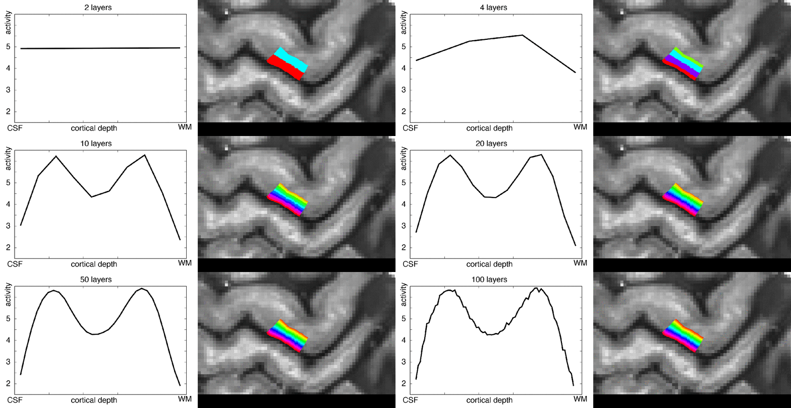
How many layers should I extract?

In this blog post, I want to share my thoughts on the number of layers that should be extracted from any given dataset. I will try to give an overview of how many layers are usually extracted in the field, I’ll describe my personal choices of layer numbers, and I will try to discuss the challenges of layer signal extraction along the way.

Continue reading “How many layers should I extract?”

Registration of high-resolution data

In this blog post Sri Kashyap and I describe how to deal with the registration of high-resolution datasets across days, across different resolutions, and across different sequences.

I am particularly fond of the following two tools: Firstly, ITK-SNAP for visually-guided manual alignment and secondly, using ANTs programs: antsRegistration and antsApplyTransforms.

Continue reading “Registration of high-resolution data”

Quick example of cortical unfolding in LAYNII

Update June 2021: There is a new and more comprehensive 3D-supported LayNii Program for cortical unfolding. Please see https://thingsonthings.org/ln2_multilaterate/

The blog post below is kept for archiving purposes: 

In this Blog post, I seek to describe a quick example of how to analyse high-resolution data across layers and columns with LAYNII.

Continue reading “Quick example of cortical unfolding in LAYNII”

Quick analysis pipeline of getting layer fMRI profiles without anatomical reference data

This is a step-by-step description on how to obtain layer profiles from any high-resolution fMRI dataset. It is based on manual delineated ROIs and does not require the tricky analysis steps including distortion correction, registration to whole brain “anatomical” datasets, or automatic tissue type segmentation. Hence this is a very quick way for a first glance of the freshly acquired data.

This post shows how you can get from activation maps to layer-profiles in 10 min. In a quick and dirty way.

The important steps are: 1.) Upscaling, 2.) Manual delineation of GM, 3.) Calculation of cortical depths in ROI, 4.) Extracting functional data based on calculated cortical depths.

Continue reading “Quick analysis pipeline of getting layer fMRI profiles without anatomical reference data”

Creating rim file from Freesurfer/Suma

Overview

Big steps:

  1. Manual aligment of MP2RAGE with EPI (optional when MP2RAGE is acquired in same session)
  2. ANTS alignment of MP2RAGE and EPI. (part of anatomical_maser.sh, see github)
  3. Running Freesurfer on MP2RAGE data in EPI space. (part of anatomical_maser.sh, see github)
  4. Using SUMA to get fine samples tissue borders in EPI-voxel space (in oblique space) (part of anatomical_maser.sh, see github) Thanks to Daniel Glen developing this workflow.
  5. Manual correction of Freesurfer GM-ribbon
  6. calculating layers from GM-ribbon in neuroDebian.

Continue reading “Creating rim file from Freesurfer/Suma”