NORDIC denoising on VASO data

Authors: Lasse Knudsen, Luca Vizioli, Federico De Martino, Lonike Faes, Dan Handwerker, Renzo Huber

This post describes the usage, capabilities and challenges of NORDIC PCA denoising on VASO data. A video presentation of this project can be found here: https://youtu.be/bbGKMTWVrJY.

NORDIC may help boost the limited detection sensitivity of laminar fMRI through thermal noise suppression. The merits and limitations of NORDIC for denoising fMRI data has previously been evaluated for BOLD acquisitions (Vizioli et al., 2021, Dowdle et al., 2023, Knudsen et al., 2023, Fernandes et al., 2023) whereas validation on VASO data is sparse (but see Huber et al., 2022 ISMRM abstract #0398, Pizzuti et al. 2022 OHBM abstract #1938, Akbari et al., 2023, Oliveira et al., 2023). Compared with BOLD, VASO comes with an additional contrast (blood-nulled images), different phase data (negative phase in CSF magnetization?), lower CNR, etc., and it is thus unclear how the publicly available matlab implementation of NORDIC should be executed. Also, it is unclear which assumptions are vital and which assumptions can be violated. E.g. is the difference between Rician and Gaussian noise domains large enough to justify the hassle of working with complex-valued data? Here, we test NORDIC across a wide parameter space to get a more intuitive feeling of how to apply NORDIC on VASO data and to identify when it fails. We characterize the quality of NORDIC denoising by metrics of:

• number of significantly activated voxels.
• spatial and temporal structure of removed noise.
• effect on beta scores with NORDIC compared to averaging
• shape of layer-profile.

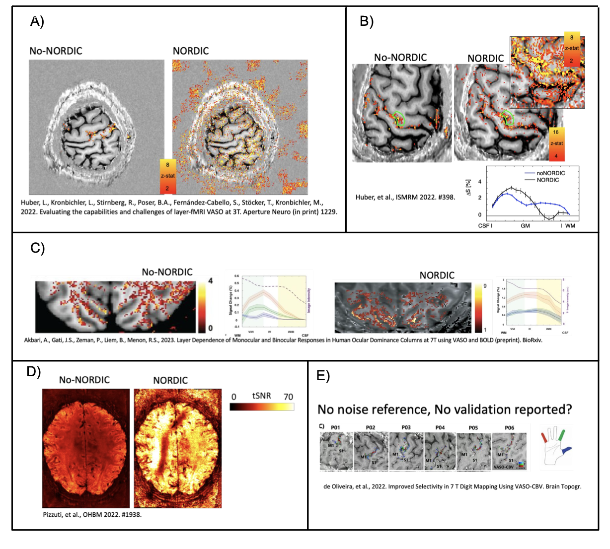
Figure 1. Example images of previous attempts to perform NORDIC with VASO. 

• Panel A). NORDIC removed the activity of interest and introduced false positive activity in patches outside the brain. It is suspected that this was due to wrong application of noise estimates with overestimated variance of multiple contrasts as one time series. In this study we want to explore the effect of noise floor estimates on NORDIC-VASO.
• Panels B-D). NORDIC boosts the sensitivity and tSNR by an order of magnitude. However, the layer-profiles of beta scores are altered. It is suspected that the noise threshold estimation might have been overestimated by the different signal composition of VASO by inappropriately applying VASO with magnitude-only data (B). Or by applying NORDIC with inappropriate coil-combined phase data (D). In this study, we want to explore the advantages and disadvantages of applying NORDIC VASO in the complex-valued or magnitude-only domain.
• Panel E) refers to the first NORDIC VASO data that are published as a peer-reviewed journal article. However, this paper does not include a validation of NORDIC and an analysis of the resulting signal responses with and without the application of NORDIC. In this study, we want to provide such validation. We aim to provide recommendations to the field on how to apply NORDIC on VASO data with minimum risk of adverse effects.

2. How does NORDIC work?

NORDIC aims to separate thermal noise from non-thermal sources (signal of interest, physiological noise, drifts, etc.) in the following steps:

1. Estimate the thermal noise-level and g-factor map with MP-PCA (Veraart et al., 2016a, Veraart et al., 2016b). Then normalize the data using the g-factor map, scaled by the estimated thermal noise level, to ensure homogenous thermal noise across the image (PCA denoising assumes identical noise distributions across voxels). 
2. Select a local patch of voxels and construct a Casorati matrix, Y, of size m-by-n where each of the m row-vectors represents the timeseries of a voxel within the patch.
3. Run principal component analysis (PCA) on this matrix using the singular value decomposition (svd). The svd breaks our data matrix down into three new matrices such that Y=USV’. The matrix V contains the n singular vectors (principal components) in its columns. These are sorted such that the first column contains the singular vector that explains most of the variance in Y, the second column contains the singular vector explaining second most of the variance etc. The first singular vector can in this context be thought of as the temporal pattern that is mostly correlated to the overall signal in Y (see Figure 2a). S is a n-by-n matrix containing the sorted singular values in its diagonal. Singular values tell how much variance is explained by the corresponding singular vector. U is a matrix of loadings and essentially provides the weights for how to linearly combine the set of singular vectors for each voxel (see Figure 2b).
4. Identify singular threshold: The trick in PCA-based denoising is to remove the singular vectors which only (or mostly) reflect thermal noise. Signals of interest will be captured in singular vectors with high singular values if it is redundantly represented across many voxels in the patch (and thus explain a relatively large portion of the overall variance), whereas any given thermal noise realization should only be truly correlated with itself under the assumption of spatial independence. Components mostly reflecting thermal noise will thus end up with the smallest singular values. NORDIC then identifies the threshold at which components with smaller singular values will be discarded (set to 0), and the matrix Y is reconstructed from the surviving components. It does so through Monte Carlo simulations; in each iteration, PCA is performed on a zero-mean Gaussian noise matrix with standard deviation matched to the thermal noise level in the measured data and of the same size as Y. The threshold is then determined as the average of the largest singular value from each iteration.   
5. Finally, the denoised patches are combined by patch-averaging and images are multiplied by the scaled g-factor map to reverse the normalization. 

The degree of noise-removal and the accuracy of denoising, i.e., how well the low-rank approximation of Y captures signal of interest, relies on: 

1. Amount of data redundancy – when more voxels have the same underlying temporal signal, that signal will end up accounting for more variance and thus be easier to separate from noise components. 
2. Number of timepoints – The more timepoints we have, the more principal components (with non-zero singular values) we get. Thermal noise is inevitably distributed across all components, and more components thus better allow for binning into signal versus noise components. 
3. Number of voxels in the patch – more is better if all else is equal, but when the patch grows, we also include more different variations of signals and more components will be needed to capture it thus counteracting 2). 
4. CNR – the stronger the response relative to the noise, the easier they are to separate. 

See Veraart et al., (2016a, 2016b); Zhu et al. (2022); Olesen et al., (2022), for further detail.

3. How should NORDIC be applied to VASO?

The VASO contrast is cerebral blood volume (CBV)-weighted, and is believed to have high spatial specificity towards microvasculature. CBV-weighting is obtained by applying an inversion pulse followed by image readout around the blood-nulling time, and the fMRI-signal will thereby decrease in proportion to increases in CBV. These so-called nulled images are interleaved with regular BOLD images (not-nulled images), which can be used to correct for positive BOLD contrast counteracting the negative CBV contrast in the nulled images (see details in Huber et al., 2014).

As mentioned above, it is somewhat unclear how NORDIC should be applied to VASO data due to, e.g., differences in contrasts, signal to noise levels, response magnitudes, etc. Therefore, we first evaluated a comprehensive spectrum of different implementations of NORDIC. These were explored with the publicly available matlab implementation of NORDIC. Questions that we wanted to address were:

1. Should nulled and not-nulled volumes be denoised combined or separately? In the “combined” versions, NORDIC was applied to the full time series where odd volumes are nulled and even volumes are not-nulled. For “separate” versions, the time series were split into nulled or not-nulled before denoising was applied to either of these individually. On one hand, the combined version has the advantage of having twice the number of volumes which should improve the ability of PCA to separate signal and noise components. On the other hand, it could be that the number of necessary components needed to describe the signal may more than double in the combined case due to interactions between VASO and BOLD, and thereby make it harder for PCA to dissociate signal and noise. Also, although nulled and not-nulled images should have the same thermal noise levels, the g-factor and noise-level estimation could perhaps be hampered due to differences in CNR?
2. With or without an appended noise volume? The publicly available matlab implementation of NORDIC allows the user to input a noise-only volume (typically acquired by the end of the run using the same sequence, but with the amplitude of the RF-pulse set to 0). After g-factor normalization, the thermal noise level can be measured from this volume as the variance across space. If no noise-volume is appended, the noise-level is estimated from the data using MP-PCA. The former option may theoretically be preferred as it represents a more direct way of getting the threshold. Here we wanted to test this empirically.      
3. With complex-valued versus magnitude only data? NORDIC can be applied using both magnitude and phase images (referred to here as complex versions) or magnitude images only (ARG.magnitude_only=1). The complex-valued versions should theoretically have an advantage, partly because the data redundancy that low-rank denoising relies upon is increased when utilizing both the magnitude and phase information, and partly because the real and imaginary parts fulfill the assumption of Gaussian distributed noise whereas magnitude images have a Rician noise distribution. The Rician distribution approaches a Gaussian shape when tSNR becomes sufficiently high, and we thus tested whether inclusion of phase-images make a large difference in practice or if one can get away with just using magnitude images.

We tried all 2^3=8 combinations on a 3T segmented multi-echo VASO dataset with 0.9 mm isotropic resolution (here we only used the first echo). The paradigm was 6 12-min runs of block-designed simultaneous visual stimulation and bilateral finger tapping (see details in Huber et al., 2022). We found this dataset ideal as it allowed us to test NORDIC in a thermal noise dominated regime with relatively low CNR, where NORDIC is most needed. It also presents a challenging test-case since the success of low-rank denoising methods is CNR dependent. Furthermore, 72 minutes of functional data provided a fairly good ground-truth estimate at the single-voxel level, and visual+motor stimulation activates large patches of cortex thus allowing extensive voxel-averaging, resulting in fairly good single-trial ground truth estimates. For all versions, NORDIC was applied to each run individually with the default isotropic patch size: k x k x k, where k=(num_TRs*11)^(⅓) rounded to the nearest integer. 

Note that the publicly available implementation of NORDIC comes in two flavours; “NORDIC.m” requires a noise-only volume and a g-factor map as inputs. The other flavour, “NIFTI_NORDIC.m”, estimates the g-factor from the data itself (more details are available at the link below from which NORDIC can be downloaded). For this blog post, we used and will focus on the NIFTI_NORDIC flavour (https: //github.com/SteenMoeller/NORDIC_Raw, v1.1, commit 74999d6), as it can be readily applied to a broader range of data sets (but see section 5 “Effect of g-factor estimation method” where the NORDIC.m flavour was explored). 

Data was extracted from a large ROI covering both visual and sensorimotor cortex. Laminar profiles were extracted from a relatively small ROI in visual cortex (data upsampled to 0.2 mm iso) (Figure 3). 

3.1 Amount of noise removal

tSNR and t-value maps provide a measure of the degree of noise-removal, and based on these alone, the complex-valued versions with the appended noise-volume seem to provide more efficient denoising, whereas the remaining versions are close (Figure 4). Even for these latter versions, NORDIC approximately doubled tSNR and increased the average single-voxel t-value from ~1.5 to ~2.5, which could be translated into e.g., shorter scan durations, higher resolutions, or allow for paradigms with lower CNR.

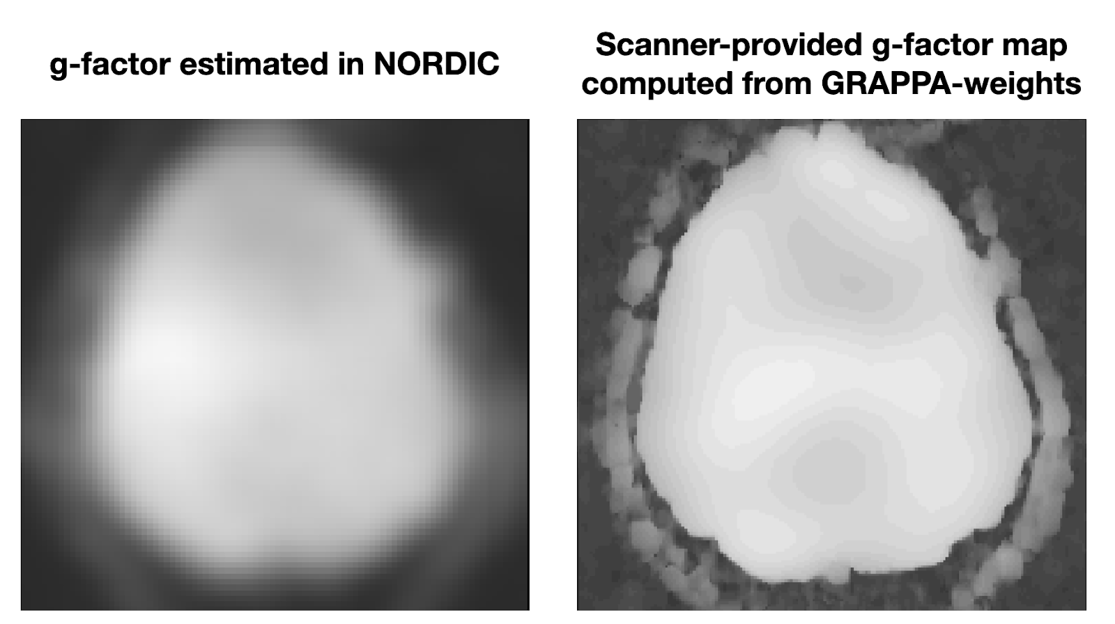
The patches of large tSNR-values outside the brain for magnitude-only versions – are they perhaps the result of denoising breaking down in areas with low SNR where the noise-distribution is non-gaussian for magnitude data? This would make sense as they are not there for complex versions where the thermal noise distribution is not a function of signal intensity. In that case, however, we would expect it to show up more widely and in a less organized manner. A complementary explanation could be that the g-factor map is expected to have fairly sharp edges at the borders of the brain, which cannot be captured by the default 14x14x1 patch size for g-factor estimation (notice the smoothness in example below taken from another dataset where “true” g-factor maps were available, Figure 5), which may result in inaccurate noise-level estimates in these areas. In any case, it does not seem to be an issue inside the brain.

3.2 Signal intactness after denoising

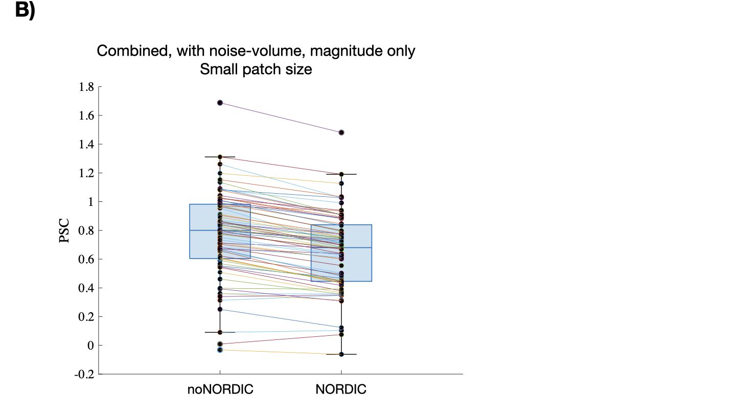
If NORDIC only removes thermal noise, the average percent signal change across ROI voxels should be unaltered (the ROI has over 7000 voxels and thermal noise should thus be practically eliminated after averaging). Figure 6A shows boxplots of single-trial percent signal changes computed from average time series across voxels in the ROI. All the combined versions have a clearly reduced percent change suggesting that NORDIC should preferably be performed on nulled and not-nulled time series separately. Since the patch-size depends on the number of timepoints, we considered the possibility of the patch perhaps being over-sized for combined versions. However, the bias seems to prevail also when patch size was set to something smaller (N=784) than for even the separate versions (N=1728) (Figure 6B).

With the above approach to assess bias, signal removal could be masked if the percent signal change is reduced towards 0 for both positive and negative responses. This motivated another plot of single-voxel trial-averaged (N=72) percent signal changes with NORDIC as a function of the noNORDIC value (Figure 7). If only thermal noise is removed, the regression line (red) should line up with the identity line (blue) (slope=1, intersection=0). The slope is smaller than 1 in all versions suggesting some bias towards 0. As in Figure 6A, the bias is largest for combined versions and is smallest for version “separate-withNoiseVolume-magnitudeOnly”, closely followed by the “separate-withoutNoiseVol” versions.

3.3 Laminar profiles

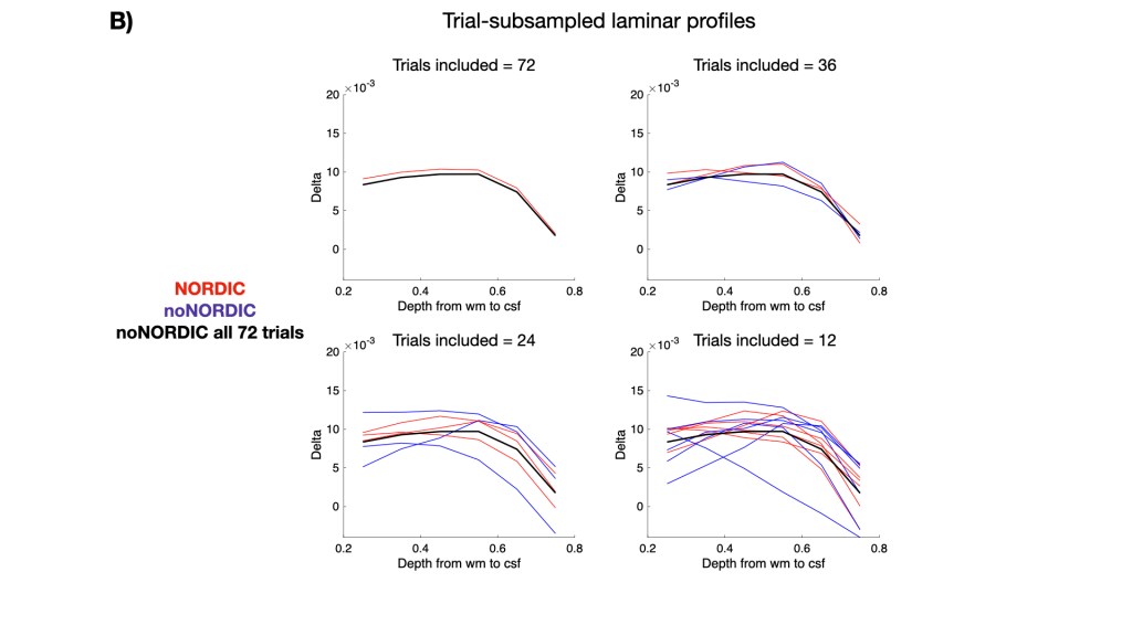
Figure 8A shows laminar profiles of each version. Ideally, NORDIC profiles should largely overlap with the noNORDIC profile (considering that we average across 72 trials), but with smaller error bars. It does look pretty good for most versions (not the “combined, with noise-vol, complex” version), suggesting that robust estimation of laminar profiles can be done with fewer trials when using NORDIC. This is illustrated in Figure 8B showing profiles with different degrees of trial-subsampling. Subsampled noNORDIC profiles already start breaking down at 24 trial averages, whereas NORDIC profiles seem quite stable even at 12 averages.  

3.4 Intactness of temporal structure

In addition to testing for changes in response magnitude, we further evaluated whether NORDIC altered the temporal structure of single-trial responses (Figure 9), by 1) plotting the voxel-averaged percent signal change as a function of trial number, and 2) plotting the autocorrelation function for this “trial-timeseries”. The versions with the largest bias in percent signal change (Figures 6-7) of course have a reduced mean, but the temporal pattern of trial variability does not seem to change after NORDIC. Also, the autocorrelation function is largely identical with and without NORDIC and reminiscent of that of simulated Gaussian noise (not shown here). If NORDIC altered the variability across trials (reduced variability is expected at the single-voxel level but not after averaging across >7000 voxels), it would bias our t-values (on top of the bias induced by response magnitude alterations), but that does not seem to be the case.

3.5 Does the removed part look thermal?

Our final test of whether NORDIC only removes thermal noise was made by computing an image of the mean difference time series, i.e., NORDIC minus noNORDIC, reflecting what is removed by NORDIC (Figure 10).  Note that for all versions there seems to be some structure in the periphery, but within the brain the difference-images look like unstructured random noise scaled by the g-factor (as expected if NORDIC does not introduce blurring) (bottom row of Figure 10).

3.6 Summary

In summary, the version that seems to best preserve the signal is the “separate-withNoiseVolume-magnitudeOnly” (wrapper for running this version can be downloaded here: https://github.com/LasseKnudsen1/NORDIC-VASO), closely followed by the “separate-withoutNoiseVol”, none of which were the ones providing the largest noise-removal. This highlights that denoising performance should not be evaluated solely from the amount of noise removal; evaluation of signal intactness should also be considered. Importantly, more noise-removal is often followed by more signal-removal thus representing a trade-off between the two (see Kay 2022 for an excellent illustration), which we will look into in the next section.

4. Manipulating the tradeoff between noise removal and signal preservation

If we were forced to select a version based on the analysis above, it would be the “separate-withNoiseVolume-magnitudeOnly” as it seemed to be the best performing version in terms of removing noise while keeping the signal intact. Accordingly, we chose to move on with this version for the next analysis. Here we denoised the data with different values of ARG.factor_error. The default value of this parameter is 1, and it basically scales the originally determined singular value threshold. That is, if ARG.factor_error=1.2, the threshold is increased by 20 % and more components will be removed, resulting in more aggressive denoising. The risk, of course, is that we become more likely to also remove signal of interest. Figure 11A illustrates this by showing the ROI-average percent change as a function of this parameter. More and more signal is removed as we increase the scaling factor, but due to the additional noise-removal, we start seeing robust sensorimotor activation that was not clear for the default scaling of 1. To further emphasize the point of signal removal, we calculated the delta from the difference time series (noNORDIC minus NORDIC), i.e., the stuff removed by NORDIC. Figure 11B shows how the difference time series contains increasingly more signal when the scaling factor grows.

With this parameter, we can balance the tradeoff between noise and signal removal as we like. For example, it may be useful to push the scaling factor for functional localizers where we don’t care so much if the response magnitude is accurate, we just want to find the right region – in this way the acquisition time spend on localizer runs could be dramatically shortened and one has more time to do the actual experiment. Another example would be the acquisition of a distortion matched T1-weighted anatomical reference computed from a VASO time series, where alterations of the signals do not really matter as long as the anatomical structure is intact. 

The fact that the percent signal change is already slightly but significantly reduced at a scaling factor of 0.9 may reflect an important issue for all low-rank denoising methods; In the presence of thermal noise, the estimated principal components will always deviate from the noise-free scenario. That is, our components will always be “corrupted” to some extent such that thermal noise and signal ends up being spread out across all components (Olesen et al., 2022, Kay et al., 2022). This effect is always there, and it only becomes a matter of its extent. In many cases it may be negligible, and a lot of noise removal at the cost of very small signal reduction will be well worth it, especially in cases where no activation is detectable without denoising. 

Potential future extensions of NORDIC could account for this bias of β-values towards zero to some extent. For example, it might be possible to include the functional stimulation design itself into the decision tree of PCA to be rejected as part of the NORDIC algorithm.

With respect to the 3T data investigated here, we do find it promising that even for the present dataset where CNR is fairly low (3T VASO at submillimeter resolution), the signal reduction appears to be quite small at the default scaling factor, and when NORDIC is implemented appropriately. This also seemed to be the case in two additional VASO datasets with different field strength (7T), sequence parameters, tasks, number of volumes, participants, etc. Results from one of these datasets is shown in the section below, the other is from Huber et al. (2017) (results not shown here, but data can be downloaded at: https://drive.google.com/drive/folders/1TkoDUG1UQwd7eGw7IVSwORmRLdF5WtWm).  

5. Effect of g-factor estimation method

As mentioned above, the matlab implementation of NORDIC can either use the g-factor map provided by the scanner (NORDIC.m), which is computed by passing simulated zero-mean Gaussian noise through the GRAPPA-kernel, or the g-factor can be estimated from the input time series (NIFTI_NORDIC.m). The former should be closer to the ground-truth and may therefore be preferable. This was tested on BOLD-data in a recent ISMRM abstract where less signal removal was indeed found for the “actual” g-factor map compared with the estimated one (Pfaffenrot and Norris, #2719, ISMRM 2023). To test this for VASO, we ran a similar analysis as in section 3., but this time on a 7T dataset (0.8mm isotropic, 4 runs of bilateral finger tapping (12 min each)), where scanner-provided g-factor maps were available.

To test whether it is worth the hassle to get a g-factor map for each run (which can be a bit impractical and time-consuming) or if one can get away with reconstructing a single map at the beginning of the session, we ran NORDIC either with the same g-factor for all runs (first run) or with run-specific maps. The current version of NORDIC.m can only be applied on complex data and with appended noise-volumes, so to most directly evaluate the effect of actual vs estimated g-factors, we also ran NIFTI_NORDIC.m with appended noise-volumes and on complex data. To test whether these versions were preferable compared with the version recommended in section 3, we also ran NIFTI_NORDIC with appended noise-volumes but on magnitude-only data.

All results (Figure 12) were extracted from a large ROI covering the hand knob of M1 in both hemispheres (ROI for laminar profiles only covered the hand knob in the left hemisphere). First, activation maps, percent change evaluations, and laminar profiles appear highly similar between using the same or run-specific g-factor maps (Figure 12), suggesting that one does not necessarily have to bother with computing g-factor maps for every run. This was the case despite large across-run motion which resulted in noticeable g-factor differences across runs (Figure 13). Second, the same can be said when comparing NORDIC.m versions with the complex-valued NIFTI_NORDIC.m version, suggesting that denoising is not wildly sensitive to (small) inaccuracies in g-factor estimates (although some local differences can be seen, for example, in the tSNR maps). Third, all these versions had some signal-removal, which is mostly evident from the scatter plots in Figure 12. This problem was largely gone for the NIFTI_NORDIC.m magnitude-only version (the “winner” from section 3), but that version also had less noise-removal (~50% tSNR increase compared with >100% increase for the complex versions).

6. Potential points in future studies to evaluate, optimize and extend NORDIC.

• If NORDIC removes part of the signal, then averaging across runs still has some advantages compared to NORDIC. This would also mean that combining the two approaches does not benefit you twice in some cases.
• In single-participant analysis, the reduction in effect size (β, percent signal) can come with a much larger reduction in variability – this is why in the beginning, we see that despite the drop in percent signal, the “combined-withNoiseVol-complex” version gives the largest benefit in t-values. However, in multi-participant analyses this issue might be more tricky. The reduction in effect size will not always be paralleled by a stronger reduction in variability, as NORDIC does not necessarily strongly affect the variability across subjects. Thus, the reduction in percent signals can be problematic, as it can affect differences between task conditions. Seen this way, NORDIC has all the same bias-variance trade-offs present in many other processing and denoising tools. It reduces variance in the individual dataset at the cost of some bias (towards zero). Generally, reducing noise is advantageous but there is a point where too much bias becomes an issue (think of typical ML examples).
• We believe that it could make sense to focus future extensions of NORDIC onto the interaction of the design with the NORDIC efficiency. It might become advantageous to solely remove PCs that have zero correlation with the task design. However, such an approach might come along with further implications. E.g., what happens to transit responses in block design studies after NORDIC?
• Overall, the more complicated endeavour is to make sure that the removed signal is not biased in some way between conditions (i.e. removing more of one condition compared to another). Based on the results shown here, there might be potential mechanisms, in which this could happen at some point. This would mean that NORDIC would not only remove a part of the main effect, but also affect the differential effects more than just making them smaller. 

7. Conclusion

Based on the present evaluation, we suggest that, for VASO, NORDIC is executed on nulled and not-nulled images separately, that a noise-only volume is included, and that only the magnitude data is used. This version seemed to best preserve the underlying signal and did come with a large reduction in thermal noise thus alleviating CNR limitations in submillimeter VASO acquisitions. Future extensions of these evaluations across more participants and more experimental setups will help to increase the generalizability of these findings. Accordingly, our message is not that e.g., complex-valued denoising should be generally avoided, but rather that the “separate-withNoiseVolume-magnitudeOnly” implementation seems to be a fairly safe way of improving CNR in VASO data. This version also has the advantage of being easily implementable since nulled and not-nulled time series typically come as separate time series off of the scanner, and no phase-images are needed.  

8. Acknowledgements

We want to thank Steen Moeller, Viktor Pfaffenrot, Alessandra Pizutti, and Tyler Morgan for your helpful input and discussions.

9. References 

Akbari, A., Gati, J. S., Zeman, P., Liem, B., & Menon, R. (2023). Layer Dependence of Monocular and Binocular Responses in Human Ocular Dominance Columns at 7T using VASO and BOLD. BioRxiv. https://doi.org/https://doi.org/10.1101/2023.04.06.535924

​​de Oliveira, Í. A. F., Siero, J. C. W., Dumoulin, S. O., & van der Zwaag, W. (2023). Improved Selectivity in 7 T Digit Mapping Using VASO-CBV. Brain Topography, 36(1), 23–31. https://doi.org/10.1007/s10548-022-00932-x

Dowdle, L. T., Vizioli, L., Moeller, S., Akçakaya, M., Olman, C., Ghose, G., Yacoub, E., & Uğurbil, K. (2023). Evaluating increases in sensitivity from NORDIC for diverse fMRI acquisition strategies. NeuroImage, 270, 119949. https://doi.org/10.1016/j.neuroimage.2023.119949

Fernandes, F. F., Olesen, J. L., Jespersen, S. N., & Shemesh, N. (2023). MP-PCA denoising of fMRI time-series data can lead to artificial activation “spreading.” NeuroImage, 273, 120118. https://doi.org/10.1016/j.neuroimage.2023.120118

Huber, L., Ivanov, D., Krieger, S. N., Streicher, M. N., Mildner, T., Poser, B. A., Möller, H. E., & Turner, R. (2014). Slab-selective, BOLD-corrected VASO at 7 Tesla provides measures of cerebral blood volume reactivity with high signal-to-noise ratio. Magnetic Resonance in Medicine, 72(1), 137–148. https://doi.org/10.1002/mrm.24916

Huber, L., Krobichler, L., Stirnberg, R., Ehses, P., Stöcker, T., Fernandez-Cabello, S., Poser, B., & Kronbichler, M. (2022). Evaluating the capabilities and challenges of layer-fMRI VASO at 3T. BioRxiv. https://doi.org/https://doi.org/10.1101/2022.07.26.501554

Kay, K. (2022). The risk of bias in denoising methods: Examples from neuroimaging. PLoS ONE, 17(7 July), 1–19. https://doi.org/10.1371/journal.pone.0270895

Knudsen, L., Bailey, C. J., Blicher, J. U., Yang, Y., Zhang, P., & Lund, T. E. (2023). Improved sensitivity and microvascular weighting of 3T laminar fMRI with GE-BOLD using NORDIC and phase regression. NeuroImage, 271, 120011. https://doi.org/10.1016/j.neuroimage.2023.120011

Moeller, S., Pisharady, P. K., Ramanna, S., Lenglet, C., Wu, X., Dowdle, L., Yacoub, E., Uğurbil, K., & Akçakaya, M. (2021). NOise reduction with DIstribution Corrected (NORDIC) PCA in dMRI with complex-valued parameter-free locally low-rank processing. NeuroImage, 226(October 2020). https://doi.org/10.1016/j.neuroimage.2020.117539

Olesen, J. L., Ianus, A., Østergaard, L., Shemesh, N., & Jespersen, S. N. (2023). Tensor denoising of multidimensional <scp>MRI</scp> data. Magnetic Resonance in Medicine, 89(3), 1160–1172. https://doi.org/10.1002/mrm.29478

Triantafyllou, C., Hoge, R. D., Krueger, G., Wiggins, C. J., Potthast, A., Wiggins, G. C., & Wald, L. L. (2005). Comparison of physiological noise at 1.5 T, 3 T and 7 T and optimization of fMRI acquisition parameters. NeuroImage, 26(1), 243–250. https://doi.org/10.1016/j.neuroimage.2005.01.007

Veraart, J., Fieremans, E., & Novikov, D. S. (2016). Diffusion MRI noise mapping using random matrix theory. Magnetic Resonance in Medicine, 76(5), 1582–1593. https://doi.org/10.1002/mrm.26059

Veraart, J., Novikov, D. S., Christiaens, D., Ades-aron, B., Sijbers, J., & Fieremans, E. (2016). Denoising of diffusion MRI using random matrix theory. NeuroImage, 142, 394–406. https://doi.org/10.1016/j.neuroimage.2016.08.016

Vizioli, L., Moeller, S., Dowdle, L., Akçakaya, M., De Martino, F., Yacoub, E., & Uğurbil, K. (2021). Lowering the thermal noise barrier in functional brain mapping with magnetic resonance imaging. Nature Communications, 12(1). https://doi.org/10.1038/s41467-021-25431-8

Zhu, W., Ma, X., Zhu, X. H., Ugurbil, K., Chen, W., & Wu, X. (2022). Denoise Functional Magnetic Resonance Imaging With Random Matrix Theory Based Principal Component Analysis. IEEE Transactions on Biomedical Engineering, 69(11), 3377–3388. https://doi.org/10.1109/TBME.2022.3168592