Computing geometric layers and columns on continuously improving human (f)MRI data

Authors: Ömer Faruk Gülban, Renzo Huber | Date: April 2024

Chapter published here: https://www.sciencedirect.com/science/article/abs/pii/B9780128204801001881

Functional magnetic resonance imaging (fMRI) today is a common method to study the human brain. The popularity of fMRI can be explained by its versatility and accessibility to study the structure-function relationship in living humans, which has historically been challenging or impossible. One area of constant progress and excitement since the early days in fMRI is the advances in hardware, MR sequences, and software which allowed researchers to image the fine details of the human brain non-invasively. fMRI is currently capable of reaching sub-millimeter resolution, effectively transforming the MRI scanner from a macroscope into a mesoscope. While 0.8 mm isotropic voxel resolution (~0.5 μl) has become a part of the daily routine of a high resolution fMRI researcher at 7 Tesla scanners, as opposed to e.g. 3 mm isotropic voxels in conventional fMRI studies conducted at 3 T (Bollmann et al. 2020), recent developments have breached 0.37 mm isotropic resolution (~0.05 μl) (Feinberg et al. 2023). This 10 fold reduction in voxel volume promises an exciting future to observe the fine mesoscopic details such as cortical layers, columns, and vessels during changes in human brain function.

In fact, human layer fMRI ^{[We include both cortical column and layer studies done in humans using fMRI under the term layer (f)MRI.]} research was so fast paced within the last decade that the number of papers published between 1997 to 2020 has almost been matched between then and the time of writing this manuscript (Feb. 2024, see Figure 1). This turning point seems to be demarcated by multiple mesoscopic (f)MRI focused special issues published within a few years: “MRI of Cortical Layers” edited by David Norris and Jonathan Polimeni in 2018; “Neuroimaging with Ultra-high Field MRI: Present and Future” edited by Jonathan Polimeni and Kamil Uludag in 2019; “Pushing the spatiotemporal limits of MRI and fMRI” edited by Lawrence L. Wald and Essa Yacoub in 2019; and “How high spatiotemporal resolution fMRI can advance neuroscience” edited by Luca Vizioli, Essa Yacoub, Laura Lewis in 2021. Together, and when combined with a few other reviews that came soon after (Huber et al. 2019, Weldon et al. 2021), there is a wealth of reading material covering almost everything one can think of for conducting layer fMRI research.

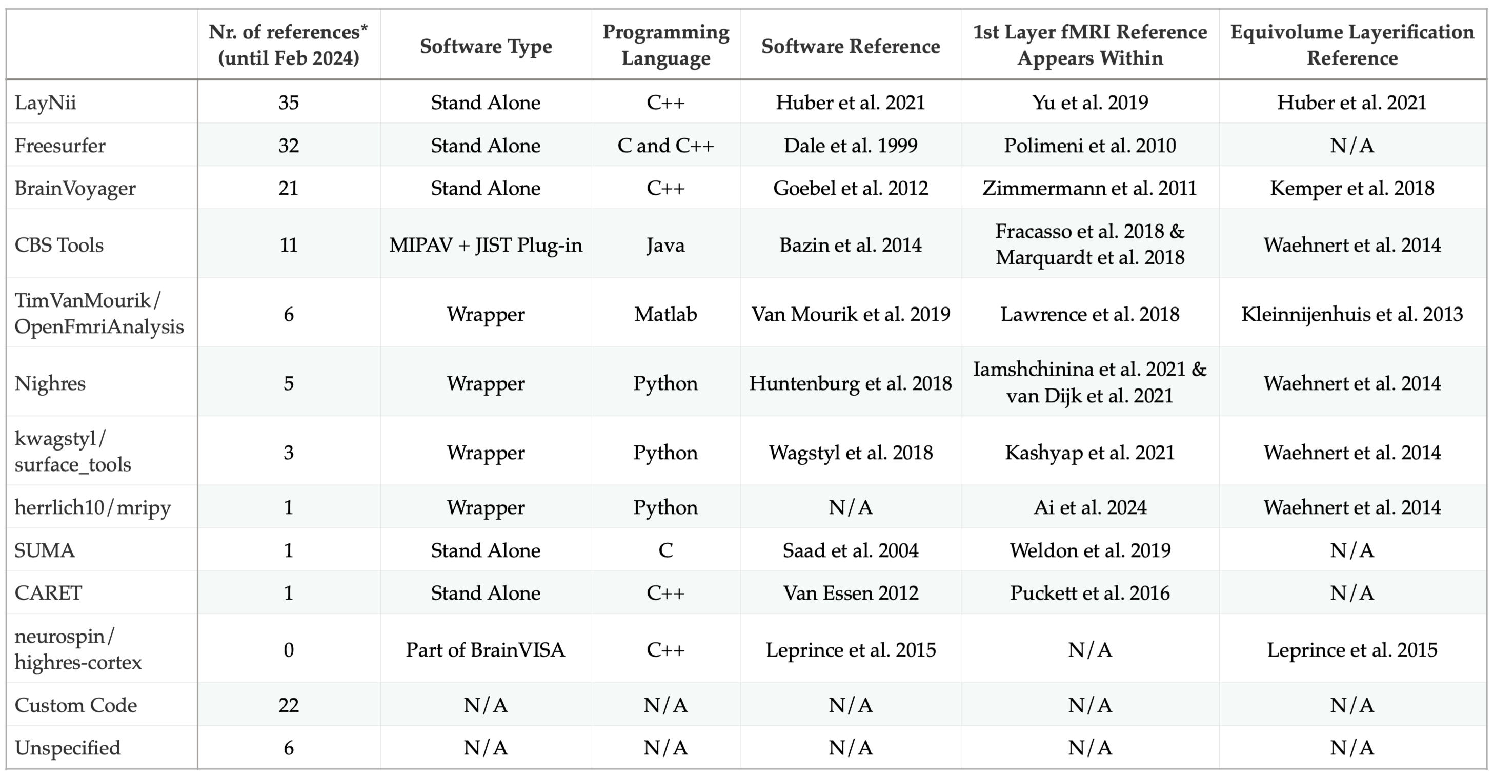
Notably, among these special issues, there are three articles that include analysis strategies” within their title (Kemper et al. 2018, Kashyap et al. 2018, Polimeni et al. 2018}. Each of these articles are written to guide the researchers on their analysis choices, providing plenty of pointers to welcome the newcomers into the field. As the authors of this text, we have to admit that we have been hard pressed to provide a unique perspective that covers a new ground. Luckily there have been a few noteworthy developments on the analysis methods within the last years. For instance, a new software package LayNii was officially born in 2019; and has been developed further by adding 3D geometric computation capabilities to provide layerification and columnification tools. Within a 4 year period of its appearance, LayNii has now become the most used cortical layer and column analysis software within the scope of human fMRI literature (Table 1). Therefore, as the main developers of LayNii, we first aim to put the recent advances into a historical context. We hope that this will improve general understanding of the essential analysis concepts that we have built upon and facilitate future developments. Our second aim is to explain what we mean by layerification and columnification and how these terms differ from the conventional neuroscientific understanding of cortical layers and columns. Our last aim is to put together the recent developments with known unknowns to elucidate future directions.

A brief history of mesoscopic neuroimaging

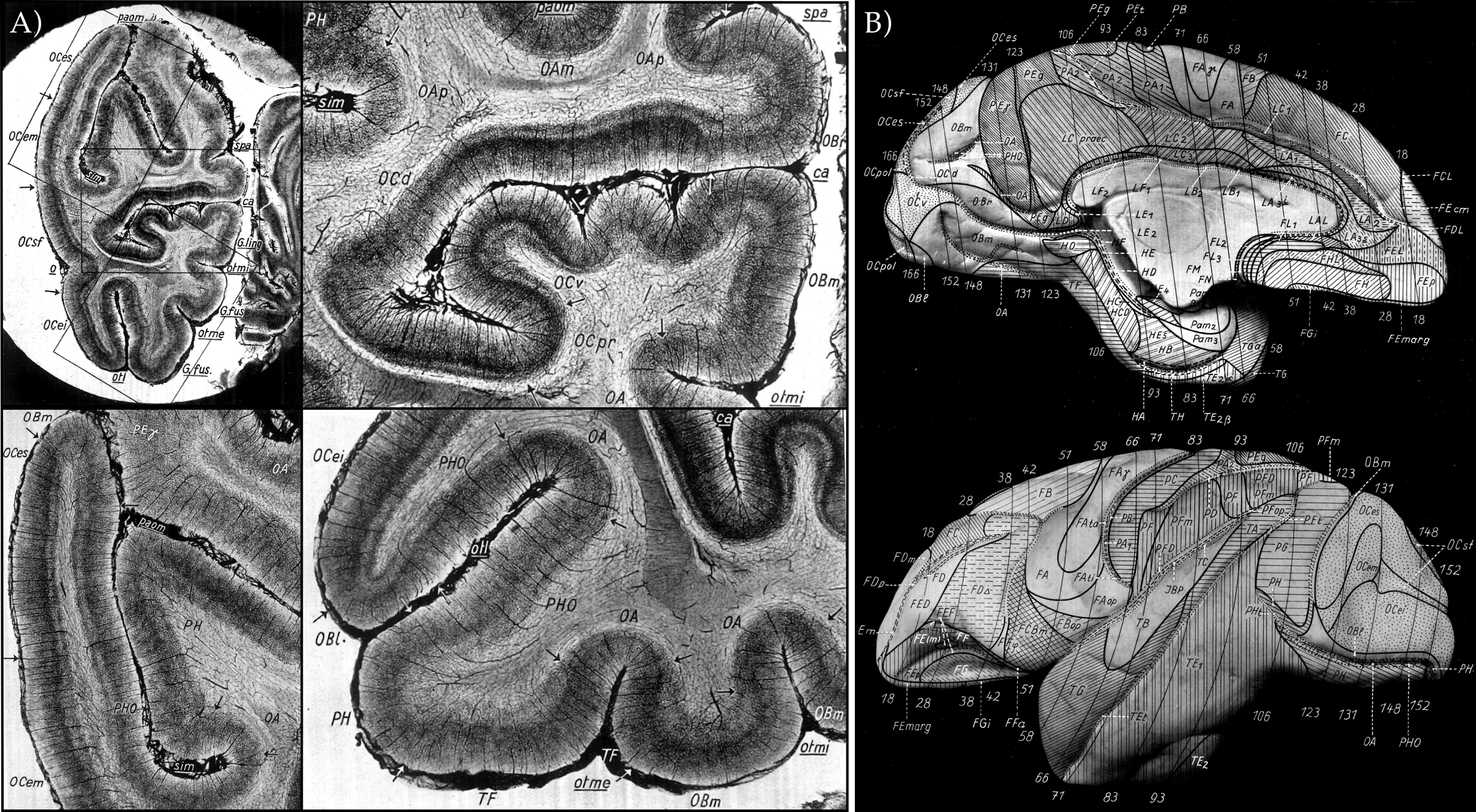
Since Francesco Gennari recognized a peculiar line running through the cortex, most easily visible on the posterior side of the ice-hardened human brains he sliced as a medical student in 1782, fine details of the cerebral cortex have been central in medical and neuroscientific research (Gennari 1782, Fulton 1937, Glickstein and Rizzolatti 1984). Particularly, in the modern era of neuroscience that has started in the late 19^th century thanks to the developments in photography and chemistry; imaging the fine details of the brain has become more and more accessible. Studying brain slices and publishing the results as photographs and sketches on paper were the primary research methods during this era. As a result, neuroscience was mainly concerned with recording, classifying, categorizing, and cataloging these fine details from the microscopic (cell shapes), to the mesoscopic (cell distributions/populations), to the macroscopic scale (sulci and gyri). Over the course of several decades, the catalog of the cortical details has grown substantially, leaving us with foundational manuscripts and atlases; each compiled for a different constituent of the cortex (Figure 2): cytoarchitecture (Triarhou 2013), myeloarchitecture (Nieuwenhuys 2013), angioarchitecture (Pfeifer 1940). Importantly, all of these architectural atlases were unified by the fact that they divide the cortical sheet into distinct layers. However, the historic laminar parcellation was not without problems.

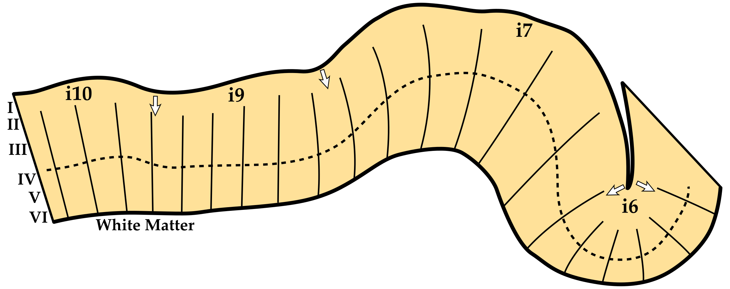
In this early era of neuroscience nearly all research was conducted by studying brain slices and publishing the results as photographs and sketches on paper. However, this two dimensional constraint on studying the slices of a brain tissue to understand e.g. its layering and how the layering changes across different brain areas required caution because the three dimensional details of the brain were hard to preserve and communicate (similar to determining the shape of a 3D object by observing its shadows). For instance, it was noted that the cortical slices are only interpretable if the cutting angle is sufficiently perpendicular to the cortex (see Figure 2.2 in Triarhou 2013). Furthermore, it was shown that even with good cutting angles, cortical layering can vary due to how the cortex bends and curves in 3D, which might have caused several researchers to delineate spurious boundaries as seen in Figure 3 (see Bok 1929, or Bok 1959, or Consolini et al. 2022 for further details). Maybe in part for this reason, the field seemed to disagree on how many cortical layers there were to begin with (see Figure 4). Therefore, it was not only critical to be aware of the sources of variance such as cortical thickness, curvature, and classification conventions but also necessary to quantify such properties; especially when studying its fine details.

Nevertheless, it seems that some consensus has been reached eventually, and we have arrived in the contemporary era of neuroscience, where six layered cortex is a given, and delineated cortical areas are largely taken for granted (for further discussionm see Nieuwenhuys 2013, Zilles 2018). In the meantime, with the discovery of magnetic resonance imaging (MRI) by Lauterbur (1973), it has become possible to image the human brain in three dimensions. Similar to the developments in photography and chemistry leading neuroscience to a new era, developments in computers and computerized image analysis lead MRI to become a dominant medical and research technology. Especially with the invention of echo planar imaging (EPI) and developments in image reconstruction; it has become possible to acquire 3D images of the brain in every few seconds (Mansfield 1977, Bernstein et al. 2004}. Together with the discovery of the blood oxygenation dependent signal (BOLD), fMRI made it possible to measure brain responses to various tasks performed by living people inside the scanner (Belliveau et al. 1991, Ogawa et al. 1992, Kwong et al. 1992, Bandettini et al. 1992). However, as fMRI only yielded clear enough images to distinguish the gray matter from the white matter, studies focused on describing what they could see at the macroscopic scale blobs of activity. Neuroscientists once again recorded, classified, categorized, and cataloged different areas of the brain in ever increasing detail, but this time based on the function rather than only the structure. Without dragging the point for too long, after around a decade and a half maturation (merely in its adolescence years), fMRI has grown bold enough to lay claims on the no man’s land: non-invasively measuring the layers of the living human brain (Ress et al. 2007, Polimeni et al. 2010, Koopmans et al. 2010)^{[However, see Cortical columns mapping section for the details of the first decade of layer fMRI that investigated ocular dominance columns in human V1.]}. This was something truly exciting, because no one could ever study living humans as they would have done with living animals, inserting electrodes into the cortex to measure activity at different layers and columns in different areas. However, before we summarize the applications of layer fMRI, it is important to put into perspective the MR data acquisition developments that paved the way for neuroscientists.

Data acquisition developments

We divide the layer fMRI developments in four partly-overlapping decade-long themes: Hardware development, contrast development, readout development, and streamlining (Figure 1). Here, we briefly summarize each period and give limited number of pointers. Readers looking for a detailed overview is invited to refer to Bollmann and Barth 2020 review.

Hardware development period: A few years after the first human fMRI results in the 90’s, the development of MR methods began to push resolutions into the mesoscopic regime (sub-millimeter). The initial decade of MR methods development saw significant advancements in ultra high field 7 T scanners and multi-channel RF coils (Ugurbil 2014). Interestingly, fMRI played a crucial role in driving such hardware developments during this period. Although 7 T scanners have now evolved into clinical scanners, their original conceptualization and development were geared for fMRI.

Contrast development period: By the 2010s, hardware development had largely subsided. Even today, nearly all layer-fMRI studies utilize the same hardware configuration that had been established in 2010: the Siemens 7Ts equipped with body gradients and a 32ch Nova RF coil. Between 2005-2015, further MR development shifted towards layer-fMRI optimized contrasts, such as GE-BOLD (Koopmans et al. 2011), SE-BOLD (Yacoub et al. 2005), 3D-GRASE (Feinberg et al. 2008), SS-SI-VASO (Huber et al. 2014), etc. Debates were common in the field to identify the optimal sequence, balancing localization specificity and functional detection sensitivity (Huber et al. 2019, Koopmans et al. 2019, Bollmann and Barth 2020). However, instead of determining the optimal sequence, researchers now lean towards using combinations of methods depending on the neuroscientific question and the experimental design.

Readout development period: From 2014 onwards, fMRI contrast mechanisms mentioned above saw no major further innovations. Rather, the focus of layer-fMRI development shifted towards those MR sequence modules that are responsible for spatial encoding. Specifically, MR development concentrated on combining mesoscale fMRI with emerging readout advancements, including SMS (Vu et al. 2017), accelerated 3D-EPI (Huber et al. 2018), multi-shot EPI segmentation (Berman et al. 2021, Huber et al. 2021), and intelligent combinations of multi-shot and CAIPI undersampling (skipped-CAIPI (Stirnberg et al. 2021), EPTI (Wang et al. 2019), EPIK (Yun et al. 2022), T-HEX (Engel et al. 2021), stack of spirals (Valsala et al. 2024), and so on …

Streamlining period: By 2018, layer fMRI became more stable, with better understanding and mitigation of noise sources (GRE-GRAPPA, and DPG) (Viessmann et al. 2021). With this, a growing number of layer-fMRI papers were solely dedicated to neuroscience (Figure 1). During this time, data acquisition and analysis methods were no longer exclusive to developers; they became stable enough to be shared more widely and applied to various cognitive neuroscience-focused research questions. However, layer-fMRI had not yet evolved into a turn-key ‘user tool.’

Looking ahead, we foresee future MR developments focusing on improving signal quality across the entire brain. Pushing the field beyond cortex, towards the subcortical areas would further exploit the capabilities of the current layer fMRI developments. Additionally, there are indications that new hardware developments may once again play a significant role, particularly in terms of magnetic field strengths above 7 T (Huber et al. 2023) and specialized head gradient technologies (Feinberg et al. 2023).

Applications of layer fMRI

While layer fMRI to study the layers and columns of the human cortex is a technology driver for new hardware and MR-sequence development, layer fMRI itself is motivated by a large range of neuroscience applications from neuronal physiology to cognitive neuroscience (papers cited within this section are illustrative and no means comprehensive).

Cortical columns mapping: The first decade of human layer fMRI studies did not primarily explore signal modulations across multiple cortical layers. Instead, the initial studies focused on mapping the ocular dominance columns within the human primary visual cortex (Menon et al. 1997, Menon et al. 1999, Dechent et al. 2000, Goodyear et al. 2001, Cheng et al. 2001, Yacoub et al. 2007, Yacoub et al. 2008) with an exception of Sun et al. (2007) focusing on temporal frequency dependent columns. These studies used single slice fMRI acquisitions where the 2D slice had to be aligned to the calcarine sulcus of the participants. The participants had to be preselected to have rather straight calcarine sulcus with consistent curvature variations. This column mapping era lasted for a decade until Ress et al. (2007) revealed that fMRI signal varies across cortical layers using 1 mm isotropic voxels at 3 T using 3D data acquisition. Truong et al. (2009), Koopmans et al. (2010), Polimeni et al. (2010) have followed by studying cortical layers using higher resolution imaging at higher field strengths. From this point onward, studying cortical layers instead of the columns became much more popular. However, cortical columns mapping did continue, in the striate cortex (Shmuel et al. 2010, DeHollander et al. 2021, Akbari et al. 2023, Haenelt et al. 2023}, the extrastriate cortex (Goncalves et al. 2015, Nasr et al. 2016, Tootell et al. 2017, Tootell et al. 2021, Fracasso et al. 2021, Kennedy et al. 2023, Ai et al. 2024), motion sensitive area hMT (Zimmermann et al. 2011, Schneider et al. 2019, Pizzuti et al. 2023), and auditory cortex (DeMartino et al. 2015, Moerel et al. 2018).

Neurovascular coupling characterization: Excitatory and inhibitory neural populations are differently distributed across the cortical layers and are expected to engage vascular responses via different neurovascular coupling mechanisms across parenchymal microvessels and pial macro vessels. Thus, many of the early neuroscience questions that were addressed with human layer-fMRI studies investigated positive and negative fMRI responses across transient and sustained periods (Goense et al. 2012). Many applications utilized layer-fMRI methods to characterize the cortical vascular anatomy as well as its response properties. (Huber et al. 2014, Siero et al. 2011, Siero et al. 2013, Siero et al. 2015, Fracasso et al. 2018, Dresbach et al. 2023, Dresbach et al. 2024). Those studies provide a detailed picture of the laminar fMRI signal generation and its dependency to spatio-temporal responses in large draining veins. With the emerging evidence that draining vein biases and physiological noise from cerebrospinal fluid (CSF) pulsation is largely confined to the pial vasculature (Olman et al. 2007, Koopmans et al. 2010, Polimeni et al. 2010), layer-fMRI tools became relevant to address questions on low resolution brain patterns. As such, even in studies that do not aim to capture laminar signal changes, layer-fMRI acquisition and analysis was helpful to mitigate biases that are present in low resolution fMRI (e.g. physiological noise, signal leakage across gyri, orientation bias) (Polimeni et al. 2010, Blazejewska et al. 2019, Viessmann et al. 2019, Kurzawski et al. 2022}. Furthermore, several neurovascular coupling studies also progressed towards understanding, building, calibrating, validating, and applying biophysical models of models of unwanted vein signals (Heinzle et al. 2016, Markuerkiaga et al. 2016, Havlicek et al. 2019, Marquardt et al. 2018, Marquardt et al. 2020, Markuerkiaga et al. 2021, Stanley et al. 2021, Huang et al. 2021).

Cortical circuitry: Laminar connectivity in hierarchically organized brain systems generally adheres to the canonical micro-circuit, with feedback terminating in superficial and deeper layers, while feedforward input terminates in middle layers (Felleman & Van Essen 1991). This model allows layer-fMRI to investigate hierarchical processing across bottom-up sensory input and top-down modulations. While earlier investigations exist (Olman et al. 2012, Muckli et al. 2015, Kok et al. 2016}; higher level cognitive questions are becoming more frequently studied using layer fMRI (Figure 1). Specific examples include: mental imagery (Persichetti et al. 2020, Turner et al. 2016), mental predictions (Yu et al. 2019, Thomas et al. 2023), prediction error propagation (Yu et al. 2022, Cerliani et al. 2022, Haarsma et al. 2020), attention modulations (DeMartino et al. 2015, Lawrence et al. 2019, Klein et al. 2018), crossmodal integration (Gau et al. 2020, Chai et al. 2021), etc.

Probing input-output: Aside from feedforward-feedback investigations, there are other layer models for investigating the micro-circuitry across layers. Which are also applicable in brain systems that are not strictly hierarchically organized. For instance, numerous cortical areas are anticipated to house dedicated micro-circuits across layers responsible for neural computations of cortico-cortical integration in the upper layers and output-circuits in the deeper layers. Therefore, layer fMRI allows probing different components of the micro-circuitry within the same brain area. One application of layer-fMRI was to investigate these circuits in the prefrontal cortex as done by (Finn et al. 2019), as well as in the motor cortex (Huber et al. 2017, McColgan et al. 2020).

Further and future applications: Anticipating increased ease of use of layer fMRI, we expect its gradual expansion into higher-order neuroimaging applications, including whole brain connectome mapping (Huber et al. 2021, Pais-Roldan et al. 2023), graph theory (Kotlarz et al. 2023), psychophysiological interaction analysis (Sharoh et al. 2019), computational cognitive model testing (Koster et al. 2018), multivoxel pattern analysis (Vizioli et al. 2020), memory encoding and retrieval (Zhang et al. 2023), and so on … For more potential applications, visit www.layerfmri.com/applications.

However, before the neuroscientists tested their laminar and columnar hypotheses of brain function, each voxel needs to be put into a reference frame in relation to the inner and outer boundaries of the cortical gray matter and in relation to the neighboring voxels in three dimensional space.

Layerification: Computing a geometric reference frame for cortical layers

The act of delineating layers within the cortical gray matter is done in two ways. The first way is to classify and categorize sufficiently differentiated patterns in the data, as shown in Figure 2. This way can be considered as verbal modeling. From Figure 4, it can be seen that researchers have different ways of labeling the same data. The second way is to impose a coordinate system on the data that allows elevating the verbal models into mathematical models. This second way is what we call “layerification” with the intent of not confusing this term with the aforementioned verbal models (Figure 5). We emphasize that layerification is necessary to transform verbal models into mathematical models. For instance, after layerification one can state that the Layer IV of von Economo and Koskinas occupies between 0.5 to 1.5 mm of depth measured from the outer surface of the cortex. However, it is well known that the cortical thickness varies across the cortex, therefore the direct cortical depth measurements need adjustment to provide a more convenient coordinate system. This adjustment is to normalize the cortical depths with the local cortical thickness measurement. For example if the cortical thickness^{[We define cortical thickness as the shortest cortical distance between the closest outer and inner cortical gray matter surfaces]} is 2.5 mm, the normalized cortical depths yield 20 % and 60 %. The cortical depth measurements normalized by the local thickness are called “equidistant” measurements. Now the same numbers can be plugged into another area of the brain that has 3 mm cortical thickness, and one can check if the Layer IV of von Economo and Koskinas appears within the same range. It is crucial to indicate the origin of the layerification (e.g. 0 % indicates the white matter boundary) and the normalization method (see Figure 7 Panel G).

Layerification would have been much easier if only discounting the cortical thickness was enough to have a useful coordinate system of the cortex. However, as argued by Bok in 1929 See Bok 1959 or Consolini et al. 2022 for the English translations), local curvature and its relationship with local thickness has to be discounted as well to have a useful cortical coordinate system. This means that two cortical locations with differing equidistant descriptions might be the same area because the relative thickness of the layer varies as a function of local curvature. For instance, if both areas have the same 2.5 mm thickness, but one of them is a gyrus and the other is a sulcus, it might be the case that the differences in the equidistant layerification are explained by the local curvature. Bok argues that the cortical tissue preserves its volume when bent and curved in 3D space; therefore if one was to take units of tissue from each area, the volumes of each layer would be the same rather than the thickness of each layer measured relative to a cortical surface. Although Bok himself did not provide a formal mathematical model that embeds the concept of local curvature and thickness into a coordinate system, he realized the volume preserving principle. According to this principle, cortical thickness and curvature are simultaneously discounted to quantify the cortical layers. Currently, we have several layerification algorithms that implement Bok’s “equivolume” principle (Table 1 Column 7).

There is little doubt that equivolume layerification is a better reference frame to report laminar findings (Figure 6). However, within the context of today’s layer fMRI studies, one needs to be aware how big of a difference equivolume layerification makes versus computational drawbacks of its implementation. For instance, (Kemper et al. 2018) shows that there is a minor difference between equidistant and equivolume layerification when the underlying fMRI data resolution is 0.8 mm isotropic, which is the current standard of layer fMRI studies. One might think that if the difference is negligible, equivolume should be the prior choice because it has been repeatedly and convincingly shown to work better than the equidistant layerification on higher resolution data (Waehnert et al. 2014, Leprince et al. 2015, Huber et al. 2021). However, the implementation details matter, and there are critical details to consider. Firstly, at lower mesoscale imaging resolutions (0.5 to 1 mm isotropic), there is an inherent uncertainty delineating the inner and outer cortical boundaries due to partial voluming in voxels. Therefore, the errors that arise from such uncertainty are going to propagate through cortical thickness and curvature estimates. This is going to destabilize the equivolume layerification more than the equidistant layerification because the equivolume layerification incorporates the local curvature into the computation whereas equidistant only depends on the local thickness. In addition, it is utmost critical to highlight the importance of accurate and precise cortical gray matter segmentation, and thorough quality control. Because the segmentation inaccuracies are going to propagate through cortical thickness estimations and result in errors in both equidistant and even more in equivolume layerification. Due to the extremely high quality requirement of cortical segmentation for layerification, this processing step is currently one of the main bottlenecks of performing fully automatic layer-fMRI studies. Note that the cost of accurate and precise segmentation scales up with the brain coverage, and number of regions under investigation. For instance, whole brain layer fMRI investigation for multiple participants can reach prohibitively long segmentation quality control durations (Koiso et al. 2023). Detailed considerations on the cortical segmentation within the context of layer fMRI are deemed out of scope for this manuscript; however, interested readers are invited to refer to Gulban & Schneider et al. 2018b.

Secondly, there is a fundamental unknown in the equivolume layerification: How smooth the transitions between differently curved areas are?. Bok has delineated his unit volumes by hand on 2D images based on the apparent change of direction of the longest axis of nerve cells (Bok 1959); however, it is unknown how to extend this rule to 3D. Currently, we determine the transition smoothness heuristically (Huber et al. 2021). However, it is possible that different implementations of the equivolume layerification would result in different results because of the computation and regularization method of the cortical curvature. Interestingly, there is a way to side-step the equivolume layerification problem that seems to be employed in diffusion MRI studies. For instance McNab et al. (2013) and Gulban et al. (2018a), divide the cortex into three curvature classes: sulcal fundi, walls, and gyro crowns; to investigate estimated fiber orientation properties across cortical depths. This is done because of the well known “radial bias” in the gyri, which means that it is more likely to detect radial fibers within the gyri in contrast to sulci. The neuroscientific discussion on radial bias is outside of our scope here; however, what we are highlighting is the fact we might need to analyze and interpret our functional data across cortical curvature types to make sure that the resulting layer profiles are not biased by the curvature types.

To summarize, we expect every layer-fMRI study to eventually use equivolume layerification to establish the appropriate coordinate system that discounts the variations which has nothing to do with the variations within the cortical circuitry. However, at the current layer fMRI resolutions, benefit of the equivolume layerification might be negligible. This being said, we urge the researcher to carefully study, report, and interpret their layer profiles in the light of cortical thickness and curvature variations within and between subjects. An example simplified fMRI layerification pipeline is illustrated in Figure 7.

Columnification: Computing a geometric reference frame for cortical columns

Cortical columns are studied less frequently in humans compared to cortical layers today. Only 20 % of all mesoscopic resolution human fMRI studies to date focus on cortical columns. However, this was not the case in the early days of layer fMRI in humans. Starting with Menon and colleagues in 1997, the aptly titled article “Ocular dominance in human V1 demonstrated by fMRI” provided a template for studying fine cortical details of living human brains. For a decade, until Ress and colleagues published the first human layer fMRI profiles in 2007, the ocular dominance columns stayed in the center of attention in seven different research articles (See “Cortical columns mapping” section). At this point, we need to delineate a line separating the neurobiological versus the geometric cortical columns. The neurobiological cortical columns were proposed as fundamental computation units of the brain in the 1950s (Mountcastle et al. 1957, Hubel & Wisel 1962, 1968, Kennedy et al. 1976) and gained attention in the later half of the 20th century. However, there is an ongoing debate on the neuroscientific basis and utility of this proposal (Horton et al. 2005, Haueis 2021). This discussion is outside of our scope here. In fact, we have come up with the term “columnification” to differentiate the act of delineating geometric columns on the cortex from the ongoing neuroscientific cortical columns discussion.

Columnification, by our definition, is required by the studies on neurobiological cortical columns, but not limited to it. Anyone who is searching for a specific laminar pattern over a column of cortex, needs columnification. Upon surveying the literature, we classify three columnification types: (I) Voronoi, (II) triangular mesh, and (III) parameterized (UVD) columnification (Figure 5). Their order of appearance is determined by the amount of computation each type requires.

Voronoi columnification is similar to nearest-neighbor tessellation or k-means clustering. A set of voxels within a region of interest is subdivided into mutually exclusive and collectively exhaustive subsets, where each subset centroid is approximately equally distant to the other centroids in its proximity (see Figure 5). The difference compared to e.g. k-means clustering on the segmented cortical gray matter voxels is that the Voronoi columns follow the cortical gray matter geometry (most often the mid thickness surface) and each subset span the entire local cortical thickness. An example simplified pipeline is illustrated in Figure 8. Other examples of the Voronoi columnification can be found in Huber et al. (2017), and Persichetti et al. (2020) where motor cortex layer fMRI activity patterns are studied. Although, in these examples, the columnification is done on 2D MRI slices, in a more recent study by Kalyani et al. (2023), the 3D extension of the Voronoi columnification algorithm (LN2_COLUMNS) within LayNii is used to study the primary somatosensory finger maps. An important benefit of the Voronoi columnification is that it allows users to compress the amount of information available within the cortex. For instance, Koiso et al. 2023 applies Voronoi columnification to compress the whole brain sub-millimeter resolution fMRI data, and to conduct similarity analyses between the columnar subsets spanning the whole brain. It is important to note that Voronoi columnification does not come with an inherent neighborhood connectivity structure. Which means that even though the cortex is geometrically subdivided, it is initially unknown which subdivisions are neighboring which others. However, this is not a hard limitation. The neighborhood can be determined afterwards (e.g. see LN2_NEIGHBORS program in LayNii v2.6).

Triangular mesh columnification is the most common and also maybe the most accessible form of establishing radial connections within the cortex. Whole-brain low-resolution MRI data is often represented in 3D by leveraging the triangular mesh data structure (Dale et al. 1999, Goebel 2012). A straightforward extension of this idea is to establish the columnar geometric elements as the mesoscale resolution by moving each vertex along their normal. For instance, if the white matter surface of a brain hemisphere is represented with a triangular mesh of 60000 vertices, by moving each vertex along their normal by the local cortical thickness, a new triangular mesh representing the superficial gray matter can be generated. Both the white matter and superficial gray matter triangular meshes in this example would have the same amount of vertices. Additional triangular meshes with the same amount of vertices, can also be generated at fractions of the cortical thickness (so called “equidistant layerification”). In this situation, each vertex that moved along the thickness can be considered as a geometric column. Examples of triangular mesh columnification can be found at Nasr et al (2016) Figure 6, and de Hollander et al. (2021) Supplementary Figure 1. A well known artifact of this method is that in highly curved areas such as the gyro crowns and sulcal fundi, surface area varies drastically across the deep and superficial gray matter, resulting in over or under sampling of the voxels as well as severe geometric distortions (Kay et al. 2019) [Also see BrainVoyager documentation section “Issues with the Whole-Mesh Sampling Approach“. However, we note that this is not a hard limitation since this issue can be mitigated by optimizing the mesh computation per cortical depth. For instance, technically, each e.g. equidistant cortical layer can be re-meshed, resulting in varying amounts of vertices across cortical surface representations, but with the upside of avoiding severe sampling issues near high curvature areas. In such case, radial neighborhoods can be established to have a data structure akin to tetrahedral meshes (Botsch et al. 2010). However, as it stands today, triangular mesh columnification is not very popular.

The most advanced form of studying the fine details of the cortex is through intrinsically parametrizing it. Parametrization of the cortex in the context of mesoscopic (f)MRI means computing two additional coordinates that are orthogonal to the one computed in layerification (see Figure 9). We are going to refer to this parametrization step as UV mapping, or UV coordinates [Leveraging the available terminology from the computer graphics, where U and V stands for the intrinsic orthogonal cortical surface coordinates and XYZ are preserved for the extrinsic Carthesian coordinates that the cortex is represented within] together with the coordinate D that we compute during layerification. We refer to the intrinsic parametrization of the cortical gray matter as UVD mapping (see Gulban et al. 2022 Figure 3). Although the intrinsic parametrization was not called UVD mapping historically in the context of layer (f)MRI, there are several early examples of this type of columnification. For instance, the first columnar (f)MRI with 3D image acquisition (Zimmermann & Goebel et al. 2011, Figure 3), uses grid sampling [as implemented in BrainVoyager] to establish the UV coordinates of the human motion sensitive area MT. Together with the equidistant layerification, the UV maps of MT were then studied for revealing the columnar patterns within it. A similar flat grid visualization revealing columnar units can be found within Goncalves et al. (2015).

Here, we highlight that UV mapping is a completely different computational step that should not be confused with triangular mesh reconstructions. For instance, in the popular fMRI data analysis software the white matter triangular mesh is commonly reconstructed based on the voxel segmentation, smoothed, and inflated. For many neuroimaging applications, such inflated triangular meshes are useful to visualize sulci simultaneously with gyri.

However, it is often desired to align different brains onto each other. Commonly, a spherical coordinate system is mapped onto the triangular meshes to allow computational benefits for surface alignments (Fischl et al. 1999a, 1999b, Frost et al. 2012, 2013, Tardif et al. 2015, Gulban et al. 2020). This spherical coordinate system computation step is an example of UV mapping that establishes notions of left-right and up-down within a spherical coordinate system. In combination with triangular mesh columnification that establishes connections between vertices spanning the cortical thickness radially, this becomes an example of UVD mapping (See Kay et al. 2019, Figures 1 and 4 as examples). However, one needs to be careful about the implications of cortex parametrization. Effectively, with parametrization we are doing a similar operation to mapping the Earth’s surface onto a 2D plane, where it is a necessity to distort the local distances and angles depending on the mapping style (e.g. Mercator projection). Further discussion on this topic can be found within Balasubramanian et al. 2010. Therefore, similarly to computing the equivolume layerification over equidistant to reduce the distortions of the reference frame that does not follow the nature of our data, care must be taken to minimize UV distortions. For example, the grid sampling used in Zimmermann et al. 2011, DeMartino et al. 2013, Muckli et al. 2015, Schneider et al. 2019, only parameterize a small portion of the cortical gray matter, optimally spanning the region of interest by means of a rectilinear grid. This is advantageous in comparison to whole hemisphere parameterization because it is similar to the homolosine projection (Goode, 1925) where smaller surface areas are parameterized piece by piece to minimize projection distortions. Another recent example of this small surface area parametrization^{[implemented in LayNii as LN2_MULTILATERATE program]} can be found within Gulban et al. 2022, Huber et al. 2023, Pizzuti et al. 2023; where instead of a rectilinear grid, a geodesic disk placed at the center of an ROI is parametrized to yield UV coordinates. Currently, we are unaware of a detailed study of the distortion characteristics of small surface area parameterization methods across each other and in comparison to whole hemisphere surface parametrization. However, it is known that whole hemisphere parameterization results in large distortion within highly curved visual areas (de Hollander et al. 2021, Kay et al. 2019).

Nevertheless, once the UV coordinates are computed for each voxel (or vertex), columnification can be achieved by evaluating the samples projected to the UV space against a kernel (see Figure 9). This kernel (or also can be called window) is often parametrized by its span UV and optionally height across the cortical thickness (D coordinate). Examples of UV columnification can be found within De Martino et al. 2015. (which uses a rectangular prism kernel), and Pizzuti et al. 2023 (which uses a cylindrical kernel). A simplified example of UV columnification pipeline is illustrated in Figure 9. In addition, it is worth to noting that the complete UVD parametrization allows intracortical filtering that adapts to local cortical geodesics, offering SNR improvements for layer fMRI applications in general (see Blazejewska et al. 2019 Figure 2, and also see LayNii LN2_UVD_FILTER program as an example implementation of such filters).

In summary, 3D columnification is the computationally heavier form of layerification due to the amount of extra steps required to compute the UV coordinates (see Figure 10). In addition, columnar fMRI is a harder form of layer fMRI because the cortical patterns are not only studied across layers but also studied over the cortical landscape without a biologically defined origin of the coordinates. However, once the geometric columns are established in a discrete (Voronoi, and triangular mesh columnification), or continuous setting (UVD columnification); it allows us to investigate the cortical landscape comprehensively to quantify spatial hypotheses. For instance, several studies (De Martino et al. 2015, Schneider et al. 2019, Pizzuti et al. 2023) compute “columnarity indices” on the UVD parametrized cortex to quantify the consistency of the geometric columns using the fMRI activity patterns. As another example, Persichetti et al. (2020), surveyed across columns to investigate the consistency of the laminar activity profiles. Overall, columnification is an active area of layer fMRI that is open for further algorithmic and application developments.

Future Directions

In this blog post, we have provided our bird’s-eye view of the MR technologies developments that allowed us to study the fine functional details of the human cortex.

In the early 20^th century, developments in photography hardware and tissue staining techniques led to rapid progress for investigating the human brain structure. Similarly, in the three decades of human fMRI to today, MRI hardware and software developments have led to rapid progress for investigating the living human brain structure and function. With new acquisition techniques, image contrasts, and analysis methods, for the first time in human history, we have created a mesoscope to observe the living human brain non-invasively. During the earlier days of this invention, developers had to become neuroscientists to test their methods on the well known neuroscientific findings (e.g. ocular dominance columns), while later, neuroscientists had to become methods developers to improve the acquisitions and analysis strategies. Thanks to this interdisciplinary back and forth, today we are in the midst of a relatively large explosion of the layer fMRI application studies where the field is moving beyond the primary sensory areas. We speculate that maybe a part of this movement should be attributed to improved accessibility of fMRI data acquisition, together with availability of streamlined data analysis methods. Although three decades might seem a long time for those doing layer fMRI, our field is still taking its baby steps to transition from a methods development field to a cognitive neuroscience field that contributes in understanding “how the human brain works”. And even beyond neuroimaging in cognitive neuroscience, the layer-fMRI technology can become a valuable tool in a much wider spectrum of neuroscience disciplines. For example, there is a large neuroscience field that is investigating cortical microcircuits with invasive methods in animal models (direct neural recordings, electrophysiology, optogenetics etc.). As in systems neuroscience, developmental neuroscience, neuropharmacology, clinical neuroscience, and cellular neuroscience. While these tools are quantitative and precise, they are limited in brain coverage and their findings cannot be easily translated to humans. Layer-fMRI tools can help to fill this gap (Yang et al. 2021). Thus, despite its current success in cognitive neuroscience, we anticipate that the main rise of layer-fMRI is still ahead of us.

On Layerification Sampling Issues

Since the early days of layer fMRI, there has been an ongoing debate about “how many geometric layers one needs to sample”. The answers to this question range from “a few” to “anything but six” ^{[“Anything but six” refers to an effort to avoid confusion between the six geometric layers with the neurobiological ones.]} to “as many as possible”. Different groups of researchers have their own favorite answer. However, it is critical for the future of our field that we reach a better understanding of the elements that go into layerification as opposed to a consensus. Therefore, rather than giving our own favorite answer, we are going to highlight the critical elements.

Imaging resolution: There is no doubt that with the current fMRI imaging resolution at ~0.8 mm isotropic voxels, we are at the very edge of starting to detect the cortical laminar details. However, although it is clear that with higher resolution, the picture of the cortex will become clearer, the mere fact of acquiring higher precision measurements does not guarantee better understanding of our data. History has shown that even when studying the cortical layers at microscopic detail, appearance of the equivolume principle of Bok took several decades. In fact, this critical principle has been lost for half a century only to be rediscovered by Waehnert et al. (2014). If the rediscovery of the equivolume principle would not have happened, and if we would have already been imaging at much higher resolutions, we would be misattributing the laminar patterns to different cortical circuitry. Similar to how some early 20^th century neuroscientists misattributed changes in the laminar patterns to areal subdivisions (Figure 3).

Cortical thickness: It is critical to measure and report the cortical thickness for layer fMRI regions of interest. For instance, imaging resolution of 0.8 mm isotropic voxels yields different relative resolutions in the primary motor cortex compared to the primary visual cortex. The average thickness of the primary motor cortex is around 4 mm in humans whereas the primary visual cortex is around 2.5 mm (Palomero-Gallagher et al. 2019). This is very important when an fMRI researcher decides to apply imaging and analysis methods developed on the primary motor cortex to the primary visual cortex. Even though the same imaging resolution can be achieved in either area, the relative imaging resolution will be lower within the visual cortex. Similarly, laminar activity profiles from different participants and brain areas should be compared to each other in the light of their relative imaging resolution. Currently, it is not common practice to report the regional cortical thickness measurements together with layer fMRI results. Therefore, we suggest that future researchers report their regional cortical thickness measurements.

Curvature: Closely following our take on reporting cortical thickness above, we think that it is equally important to give more thought on the regional curvature measurements. We have previously described the importance of the equivolume layerification principle and how relative laminar thicknesses are affected by local curvature. It seemed that the best frame of reference to account for the curvature effects is to choose the equivolume layerification. At the same time, we also noted that for the current 0.8 mm isotropic resolution, the choice of equivolume layerification might not be so critical. Our stand on this issue might sound impractical and confusing. However, here we clarify that it is important to distinguish the choice of the reference frame from the epiphenomenon that gives rise to the imaged data. For example, as a thought experiment, a perfectly computed equivolume layerification is still going to yield differing laminar activity patterns across gyri, and sulci due to the partial voluming of each neurobiological layer with the imaging voxels. It is well known that the relative thickness of the cortical layers change with local curvature. Deep layers become thicker in the gyri but thinner in the sulci; superficial layers become thinner in the gyri but thicker in the sulci. Therefore, if one agrees that the cortical thickness is critical for the interpretation of the layer fMRI results; one must also agree that the same is true for cortical curvature. Currently, investigation of the layer fMRI activation patterns across cortical curvature types are almost non-existent. Interestingly, it seems that doing so is a standard method of analysis within the in vivo cortical diffusion MRI literature that studies the cortical fibers across layers (Gulban et al. 2018a, McNab et al. 2013). We think that future studies might shed further light on the interaction between relative laminar thicknesses and the local cortical curvature and how this affects our ability to detect and distinguish laminar activity patterns. Finally, for specific brain regions that are known to have less anatomical variability (e.g. primary motor cortex) and do not span a highly varying range of curvature we might not see different laminar profiles across individuals. However, for other areas that are sometimes located within a sulcus and other times a gyrus (e.g. such as hMT), we might see different laminar profiles.

Region of interest size: When comparing layer fMRI results across different areas and individuals, it is important to note the overall size of the regions (Kashyap et al. 2018). For instance, when plotting individual layer profiles it would be informative to note the total volume (e.g. number of voxels multiplied by the voxel size). It is known that the way the cortical areas are delineated are subject to individual differences (Sugiura et al. 2007, Rademacher et al. 2001, Frost et al. 2012). Therefore, similar to paying attention to the average cortical thickness and curvature, we need to measure and report the size of our regions of interest. Surely, a laminar activity profile that fits to our expectation coming from a small ROI should be considered against another laminar activity profile that does not fit to our expectation but comes from a much larger ROI or vice versa.

Cortex segmentation: There is no doubt that a very high quality standard must be reached with the preprocessing of the anatomical and functional data for doing layer fMRI and such details are covered elsewhere (Kemper et al. 2018, Kashyap et al. 2018, Polimeni et al. 2018). However, within the context of layerification, it is utmost critical to ensure high accuracy and precision of the cortical gray matter segmentation. Even with perfectly implemented layerification algorithms, consistent biases or strong outliers within the segmentation is going to distort the laminar activity profiles. Currently, we see that more and more papers include a segmentation quality figure and in addition share their preprocessed data. Although having a figure to show segmentation quality is useful and appreciated, it still represents a tiny portion of the 3D data and is therefore not sufficient enough to judge its quality. Therefore, we support the current ongoing efforts on data sharing and encourage widespread acceptance of it. In addition, we note that the more segmented high quality data we share, the faster and more likely it will become possible to develop novel high precision segmentation algorithms fit for our domain (Gulban & Schneider et al 2018b, Svanera et al. 2021).

Overall, we suggest the future layer fMRI studies to consider reporting their descriptive statistics showing cortical thickness, curvature, sizes of each region of interest together with their layer profiles. In addition, we encourage researchers to include pointers to the preprocessed data together with the data quality figures in order to establish confidence and eliminate segmentation bias related variability within the laminar activity profiles reported across papers.

Known unknowns of layerification and columnification

Siegfried Thomas Bok’s work focused on understanding the sources of variance behind the fine details of the cortex, with a central theme being the formalization of the equivolume principle of layerification. Although his work was originally published in German in 1929 and later rediscovered in 2014 by Waehnert and colleagues, and translated to English in 2021 by Consolini and colleagues; it is a little known fact that Bok himself has published a compilation of his papers in English 1959. Interestingly, he chose to name this book “Histonomy of the cerebral cortex” ^{[Currently this is a rare book that can only be acquired second hand or accessed from libraries]}. Some readers at this point might think that histonomy is a typo and what is meant to be written is histology, a common term that refers to studying the fine details of tissues. However, this is not a typo. It was fully intentional. In his original opening and closing chapters, Bok vividly argues about the importance of careful quantification and modeling. He contrasts astrology to astronomy, where the former is concerned with describing and interpreting the data (positions of the stars observed from earth), whereas the latter is concerned with deriving principles and laws from the same data that not only explains that data but quantifies the relations between the data points. Strikingly, Bok states that since much of the histology in his era was focused on recording, classifying, categorizing, and cataloging the observed data, he wanted to distinguish his work as “histonomy” as he primarily spent effort on getting at the principles and laws behind the observed data. Of course, histology as we know today has progressed beyond what Bok referred to, yet still, we feel that his message should be taken seriously today when doing layer fMRI. We have access to better and higher technology today that is steadily progressing towards making more accurate and precise measurement, however, the mere act of more accurate and precise measurement does not guarantee furthering our understanding of how the human brain works. Therefore, in this subsection, we are going to list our known unknowns that we feel will be useful to understand the fine cortical details that we started to resolve.

Beyond equivolume: We have referred to Bok’s equivolume principle many times in our layerification chapter. However, this does not mean that all the work is done. Although it was a significant step towards improving the reference frame, we do not fully understand the mechanism that gives rise to this rather simple principle. It is important to combine brain development studies with mathematical modeling to understand the mechanical forces that create the curvature of the cortex (Holland et al. 2018, Toro et al. 2005, Darayi et al. 2022, Demirci et al. 2022). It is conceivable that more advanced cortical curvature reference frames will be constructed to account for the geometric source of variance across the relative laminar thicknesses (Kutten et al. 2024, Younes et al. 2024).

Angioarchitecture: It is a somewhat neglected fact that the cortex is not only constituted by neurons and their connections to each other but there exists a highly convoluted and structured mesh of vessels. This mesh of vessels, the cortical angioarchitecture, is not a homogenous structure penetrating the cortex, but it has a laminar structure visible at the mesoscopic scale (Duvernoy et al. 1981). In fact, there even exists a whole brain parcellation based on the variations of the cortical laminar angioarchitecture, albeit in macaque monkeys and not yet in humans (see Figure 11). As we are doing fMRI, and as it is well known that the fMRI signal reflects the changes within the blood, the implications of angioarchitecture on understanding the sources of variance in the fMRI data are numerous. However, it is currently unknown which geometric principles the angioarchitectonic cortical layers follow. It is probably safe, but not demonstrated, to assume that they do follow the equivolume principle, as the cytoarchitectonic layers do. Therefore, a promising future direction involves combining high resolution three dimensional angioarchitectonic imaging (Lauwers et al. 2008, Keller et al. 2011, Kirst et al. 2020} to quantify the relative relations of the angioarchitectonic layers across cortical curvature in humans. In addition, cortical angioarchitecture also has a radial spatial pattern. What Duvernoy et al. (1981) calls as the “intracortical vessels” that connect the capillaries to the pial vessels (see Figure 12) are critical cortical details that we need to understand to better interpret our fMRI signal. For instance, mesoscopic intracortical vessels ascending from deep gray matter seem to converge towards the superficial gray matter (see Duvernoyet al. 1981 Figure 53 and 58). In addition, it has already been shown in animals that these radial angioarchitectonic elements have unique hemodynamic response characteristics (Silva et al. 2002, Bolan et al. 2006, Park et al. 2008, Yu et al. 2016}. These mesoscopic radial angioarchitecture elements will play a larger role in modeling and interpreting the functional activation patterns as we progress towards higher fMRI resolutions (<0.4 mm iso.).

Mesoscopic vascular MRI: In the recent years, there has been a push towards using the ultra-high-field scanners to achieve mesoscopic vascular imaging (Bernier et al. 2018, Mattern et al. 2018, Lusebrink et al. 2021, Bollmann et al. 2022, Gulban et al. 2022) reach well below 0.5 mm isotropic resolution in vivo (see Figure 12 Panel D). Therefore, considering the effects of vessels on the BOLD signal, we think that the fusion of the mesoscopic vascular MRI is going to play a bigger role in the future layer fMRI. However, it is not going to be enough to simply co-register the anatomical and functional images; we need to move towards quantification and modeling with novel analysis methods and algorithms. Initial steps that directly tap into the angioarchitectonic effects on the human layer fMRI activation patterns can be found within Kay et al. (2019), Stanley et al. (2021), Finn et al. (2021), Gomez et al. (2024), Dresbach et al. (2024).

Columnar quantification: It is clear that there are radially oriented fine details of the cortex. Some of these radial elements are mesoscopic intracortical vessels and others might be the neurobiological columns. In either way, it is critical to quantify the fMRI activity patterns across radial units of the cortex. This is particularly needed for column fMRI studies that use 3D acquisitions (as opposed to the single slice slabs used in between 1997-2008 period), and studies that sample multiple cortical layers (as opposed to only sampling the deepest layer method by (Tootell et al. 2017, Nasr et al. 2018, Tootell et al. 2021}. Starting with De Martino et al. (2015), “columnarity index” computation, there has been a few developments later in Schneider et al. (2019) and more recently Pizzuti et al. (2023) to measure the local consistency of the fMRI activation along a geometric cortical column. Moreover, a generalized form of testing a spatial laminar hypothesis might be a useful direction to quantify single or double peaked laminar activity across the cortical landscape. An early example of such spatial laminar hypothesis testing can be found in Persichetti et al. (2020, Figure 1 Panel D). In addition, we think that the earlier columnar analyses and simulations (Shmuel et al. 2010, Zimmermann et al. 2011, Chaimow et al. 2018) can be improved beyond the 2D plane to incorporate local thickness and curvature changes across the cortex ^{[An example of 3D column simulation can be found within Pizzuti et al. 2023, Figure 10 and Supplementary Figure 4.]}. Adding the spatial angioarchitecture modeling into such fMRI simulations might shed further light onto the detection of columnar structures within the cortex (Adams et al. 2015).

Final words

In this chapter, we have given our outlook on computing the geometric layer and columns of the human cortex in the context of continuously improving fMRI data. Looking back at the three decades of fMRI development, we are hopeful to see the layer and column fMRI field moving towards neuroscience application studies. Even compared to the last decade, availability and accessibility of the data acquisition and analysis tools have remarkably improved. As acquisition and analysis pipelines will continuously keep improving over the next years and decades, they will become easier to apply, they will become more accessible to wider groups of researchers, and ultimately, they will become a standard method in the toolkit of neuroscientists.

Acknowledgements

Omer Faruk Gulban is supported by Brain Innovation (Maastricht, NL). Renzo Huber is supported by the NIH Intramural Program of NIMH/NINDS (#ZIC MH002884). The software suite LayNii that is referred to in this chapter is supported by Brain Innovation as an open source project. We thank Martin Havlicek for discussions on cortex parametrization within the 2015-2019 period. Our literature tables are inspired by Kashyap 2019 (PhD Thesis) Table 1.1. We thank Tyler A. Morgan, Yawen Wang, Alessandra Pizzuti, Sebastian Dresbach, Kenshu Koiso, Lasse Knudsen, Ana Arsenovic, Johannes Franz, Kendrick Kay, Andrew Persichetti, Taylor Li, Sriranga Kashyap, Daniel Glen, Saskia Bollmann for discussions and feedback on our manuscript at various stages.

Images and animations that are not referenced above have been created by the author and licensed under CC BY 4.0 license.

References

• Adams, D. L., Piserchia, V., Economides, J. R., & Horton, J. C. (2015). Vascular Supply of the Cerebral Cortex is Specialized for Cell Layers but Not Columns. Cerebral Cortex, 25(10), 3673–3681.
• Ai, H., Lin, W., Liu, C., Chen, N., & Zhang, P. (2024, February). Mesoscale functional organiza- tion and connectivity of color, disparity, and naturalistic texture in human second visual area (preprint).
• Akbari, A., Gati, J. S., Zeman, P., Liem, B., & Menon, R. S. (2023, April). Layer Dependence
  of Monocular and Binocular Responses in Human Ocular Dominance Columns at 7T using
  VASO and BOLD (preprint). Neuroscience.
  Balasubramanian, M., Polimeni, J. R., & Schwartz, E. L. (2010). Near-isometric flattening of
  brain surfaces. NeuroImage, 51(2), 694–703.
• Bandettini, P. A., Wong, E. C., Hinks, R. S., Tikofsky, R. S., & Hyde, J. S. (1992). Time course EPI of human brain function during task activation. Magnetic resonance in medicine, 25(2), 390–7.
• Bazin, P.-L., Weiss, M., Dinse, J., Sch ̈afer, A., Trampel, R., & Turner, R. (2014). A computational framework for ultra-high resolution cortical segmentation at 7Tesla. NeuroImage, 93 Pt 2, 201–9.
• Belliveau, J., Kennedy, D., McKinstry, R., Buchbinder, B., Weisskoff, R., Cohen, M., Vevea, J., Brady, T., & Rosen, B. (1991). Functional mapping of the human visual cortex by mag-
  netic resonance imaging. Science, 254(5032), 716–719.
• Berman, A. J., Grissom, W. A., Witzel, T., Nasr, S., Park, D. J., Setsompop, K., & Polimeni, J. R. (2021). Ultra-high spatial resolution BOLD fMRI in humans using combined segmented-
  accelerated VFA-FLEET with a recursive RF pulse design. Magnetic Resonance in Medicine, 85(1), 120–139.
• Bernier, M., Cunnane, S. C., & Whittingstall, K. (2018). The morphology of the human cerebrovascular system. Human Brain Mapping, 39(12), 4962–4975.
• Bernstein, M. A., King, K. F., & Zhou, X. J. (2004). Handbook of MRI Pulse Sequences [Publication Title: Handbook of MRI Pulse Sequences ISSN: 1053-1807]. Elsevier.
• Blazejewska, A. I., Fischl, B., Wald, L. L., & Polimeni, J. R. (2019). Intracortical smoothing of
  small-voxel fMRI data can provide increased detection power without spatial resolu-
  tion losses compared to conventional large-voxel fMRI data. NeuroImage, 189(January), 601–614.
• Bok, S. T. (1929). Der Einfluss der in den Furchen und Windungen auftretenden Krummungender Grosshirnrinde auf die Rindenarchitektur. Zeitschrift fur die gesamte Neurologie und Psychiatrie, 121(1), 682–750.
• Bok, S. T. (1959). Histonomy of the Cerebral Cortex. Elsevier.
• Bolan, P. J., Yacoub, E., Garwood, M., Ugurbil, K., & Harel, N. (2006). In vivo micro-MRI of
  intracortical neurovasculature. NeuroImage, 32(1), 62–69.
• Bollmann, S., & Barth, M. (2020). New acquisition techniques and their prospects for the achievable resolution of fMRI. Progress in Neurobiology, (September), 101936.
• Bollmann, S., Mattern, H., Bernier, M., Robinson, S. D., Park, D., Speck, O., & Polimeni, J. R.
  (2022). Imaging of the pial arterial vasculature of the human brain in vivo using high-resolution 7T time-of-flight angiography. eLife, 11, 2021.06.09.447807.
• Botsch, M., Kobbelt, L., Pauly, M., Alliez, P., & Levy, B. (2010). Polygon Mesh Processing [Publication Title: Polygon Mesh Processing]. CRC press.
• Brodmann, K. (1914). Physiologie des Gehirns. In P. Von Bruns (Ed.), Neue deutsche Chirurgie (pp. 85–426, Vol. 11). Enke.
• Cerliani, L., Bhandari, R., De Angelis, L., Van Der Zwaag, W., Bazin, P.-L., Gazzola, V., & Keysers, C. (2022). Predictive coding during action observation – A depth-resolved intersubject functional correlation study at 7T. Cortex, 148, 121–138.
• Chai, Y., Liu, T. T., Marrett, S., Li, L., Khojandi, A., Handwerker, D. A., Alink, A., Muckli, L., &
  Bandettini, P. A. (2021). Topographical and laminar distribution of audiovisual processing within human planum temporale. Progress in Neurobiology,
  205(July), 102121.
• Chaimow, D., Ugurbil, K., & Shmuel, A. (2018). Optimization of functional MRI for detection, decoding and high-resolution imaging of the response patterns of cortical columns. NeuroImage, 164, 67–99.
• Cheng, K., Waggoner, R., & Tanaka, K. (2001). Human Ocular Dominance Columns as Revealed by High-Field Functional Magnetic Resonance Imaging. Neuron, 32(2), 359–374.
• Consolini, J., Demirci, N., Fulwider, A., Hutsler, J. J., & Holland, M. A. (2022). Bok’s equivolume principle: Translation, historical context, and a modern perspective. Brain Multiphysics, 3, 100057.
• Dale, A. M., Fischl, B., & Sereno, M. I. (1999). Cortical surface-based analysis: I. Segmentation and surface reconstruction. NeuroImage, 9(2), 179–194.
• Darayi, M., Hoffman, M. E., Sayut, J., Wang, S., Demirci, N., Consolini, J., & Holland, M. A.
  (2022). Computational models of cortical folding: A review of common approaches.
  Journal of Biomechanics, 139, 110851.
• De Martino, F., Moerel, M., Ugurbil, K., Goebel, R., Yacoub, E., & Formisano, E. (2015). Frequency preference and attention effects across cortical depths in the human primary auditory cortex. Proceedings of the National Academy of Sciences of the United States of
  America, 112(52), 16036–16041.
• De Martino, F., Zimmermann, J., Muckli, L., Ugurbil, K., Yacoub, E., & Goebel, R. (2013). Cortical depth dependent functional responses in humans at 7T: Improved specificity with
  3D GRASE. PloS one, 8(3), e60514.
• Dechent, P., & Frahm, J. (2000). Direct mapping of ocular dominance columns in human primary visual cortex. NeuroReport, 11(14), 3247–3249.
• de Hollander, G., van der Zwaag, W., Qian, C., Zhang, P., & Knapen, T. (2021). Ultra-high field fMRI reveals origins of feedforward and feedback activity within laminae of human ocular dominance columns. NeuroImage, 228(June 2020), 117683.
• Demirci, N., & Holland, M. A. (2022). Cortical thickness systematically varies with curvature and depth in healthy human brains. Human Brain Mapping, (January).
• Ding, S.-L., Royall, J. J., Sunkin, S. M., Ng, L., Facer, B. A., Lesnar, P., Guillozet-Bongaarts, A., McMurray, B., Szafer, A., Dolbeare, T. A., Stevens, A., Tirrell, L., Benner, T., Caldejon, S.,
  Dalley, R. A., Dee, N., Lau, C., Nyhus, J., Reding, M., . . . Lein, E. S. (2016). Comprehen-
  sive cellular-resolution atlas of the adult human brain. Journal of Comparative Neurology,
  524(16), Spc1–Spc1.
• Dresbach, S., Huber, L. (, Gulban, O. F., & Goebel, R. (2023). Layer-fMRI VASO with short
  stimuli and event-related designs at 7 T. NeuroImage, 279, 120293.
• Dresbach, S., Huber, R., Gulban, O. F., Pizzuti, A., Trampel, R., Ivanov, D., Weiskopf, N., &
  Goebel, R. (2024, January). Characterisation of laminar and vascular spatiotemporal dynamics of CBV and BOLD signals using VASO and ME-GRE at 7T in humans (preprint). Neuroscience.
• Duvernoy, H. M., Delon, S., & Vannson, J. L. (1981). Cortical blood vessels of the human brain. Brain research bulletin, 7(5), 519–79.
• Engel, M., Kasper, L., Wilm, B., Dietrich, B., Vionnet, L., Hennel, F., Reber, J., & Pruessmann, K. P. (2021). T-Hex: Tilted hexagonal grids for rapid 3D imaging. Magnetic Resonance in Medicine, 85(5), 2507–2523.
• Feinberg, D., Harel, N., Ramanna, S., Ugurbil, K., & Yacoub, E. (2008). Sub-millimeter Single shot 3D GRASE with Inner Volume Selection for T2 weighted fMRI applications at 7
  Tesla 1 [Issue: 4]. Proc. Intl. Soc. Mag. Reson. Med. 16, 37, 2373.
• Feinberg, D. A., Beckett, A. J. S., Vu, A. T., Stockmann, J., Huber, L., Ma, S., Ahn, S., Setsompop, K., Cao, X., Park, S., Liu, C., Wald, L. L., Polimeni, J. R., Mareyam, A., Gruber,
  B., Stirnberg, R., Liao, C., Yacoub, E., Davids, M., . . . Dietz, P. (2023). Next-generation
  MRI scanner designed for ultra-high-resolution human brain imaging at 7 Tesla. Nature
  Methods, 20(12), 2048–2057.
• Felleman, D. J., & Van Essen, D. C. (1991). Distributed Hierarchical Processing in the Primate Cerebral Cortex. Cerebral Cortex, 1(1), 1–47.
• Finn, E. S., & Bandettini, P. A. (2021). Movie-watching outperforms rest for functional connectivity based prediction of behavior. NeuroImage, 235, 117963.
• Finn, E. S., Huber, L., Jangraw, D. C., Molfese, P. J., & Bandettini, P. A. (2019). Layer-dependent activity in human prefrontal cortex during working memory. Nature Neuroscience, 22(10), 1687–1695.
• Fischl, B., Sereno, M. I., & Dale, A. M. (1999). Cortical surface-based analysis: II. Inflation, flattening, and a surface-based coordinate system [arXiv: 10.1006/nimg.1998.0396 ISBN:
  1053-8119 (Print)\n1053-8119 (Linking)]. NeuroImage, 9(2), 195–207.
• Fischl, B., Sereno, M. I., Tootell, R. B., & Dale, A. M. (1999). High-resolution intersubject averaging and a coordinate system for the cortical surface. Human Brain Mapping, 8(4), 272–284.
• Fracasso, A., Dumoulin, S. O., & Petridou, N. (2021). Point-spread function of the BOLD response across columns and cortical depth in human extra-striate cortex. Progress in Neurobiology, 202(March), 102034.
• Fracasso, A., Luijten, P. R., Dumoulin, S. O., & Petridou, N. (2018). Laminar imaging of positive and negative BOLD in human visual cortex at 7 T. NeuroImage, 164(February 2017), 100–111.
• Frost, M. A., & Goebel, R. (2012). Measuring structural–functional correspondence: Spatial
  variability of specialised brain regions after macro-anatomical alignment. NeuroImage,
  59(2), 1369–1381.
• Frost, M. A., & Goebel, R. (2013). Functionally informed cortex based alignment: An inte-
  grated approach for whole-cortex macro-anatomical and ROI-based functional align-
  ment. NeuroImage, 83, 1002–10.
• Fulton, J. F. (1937). A Note on Francesco Gennari and the Early History of Cytoarchitectural Studies of the Cerebral Cortex. Bulletin of the Institute of the History of Medicine, 5(10), 895–913.
• Gau, R., Bazin, P.-L., Trampel, R., Turner, R., & Noppeney, U. (2020). Resolving multisensory and attentional influences across cortical depth in sensory cortices. eLife, 9, e46856.
• Gennari, F. (1782). De Peculiari Structura Cerebri. Nonnullisque ejus morbis. Ex Regio Ty-
  pographeo, Parma., 44(0).
• Glickstein, M., & Rizzolatti, G. (1984). Francesco Gennari and the structure of the cerebral cortex. Trends in Neurosciences, 7(12), 464–467.
• Goebel, R. (2012). BrainVoyager–past, present, future. [arXiv: 4]. NeuroImage, 62(2), 748–56.
• Goense, J., Merkle, H., & Logothetis, N. K. (2012). High-Resolution fMRI Reveals Laminar Differences in Neurovascular Coupling between Positive and Negative BOLD Responses.
  Neuron, 76(3), 629–639.
• Gomez, D. E. P., Polimeni, J. R., & Lewis, L. D. (2024, February). The temporal specificity of BOLD fMRI is systematically related to anatomical and vascular features of the human brain (preprint). Neuroscience.
• Goncalves, N. R., Ban, H., Sanchez-Panchuelo, R. M., Francis, S. T., Schluppeck, D., & Welchman, A. E. (2015). 7 tesla FMRI reveals systematic functional organization for binocular disparity in dorsal visual cortex. The Journal of neuroscience : the official journal of the Society for Neuroscience, 35(7), 3056–72.
• Goode, J. P. (1925). The Homolosine Pprojection: A New Device For Portraying The Earth’s
  Surface Entire. Annals of the Association of American Geographers, 15(3), 119–125.
• Goodyear, B. G., & Menon, R. S. (2001). Brief visual stimulation allows mapping of ocular
  dominance in visual cortex using fMRI. Human Brain Mapping, 14(4), 210–217.
• Gulban, O. F., Schneider, M., Marquardt, I., Haast, R. A. M., & De Martino, F. (2018a). A scalable method to improve gray matter segmentation at ultra high field MRI. PloS one, 13(6), e0198335.
• Gulban, O. F., De Martino, F., Vu, A. T., Yacoub, E., Ugurbil, K., & Lenglet, C. (2018b). Cortical fibers orientation mapping using in-vivo whole brain 7 T diffusion MRI. NeuroImage, 178(December 2017), 104–118.
• Gulban, O. F., Goebel, R., Moerel, M., Zachlod, D., Mohlberg, H., Amunts, K., & De Martino,
  F. (2020). Improving a probabilistic cytoarchitectonic atlas of auditory cortex using a
  novel method for inter-individual alignment. eLife, 9, 1–29.
• Gulban, O. F. (2020). Imaging the human auditory system at ultrahigh magnetic fields [Doctoral dissertation, Maastricht University] [ISBN: 9789463809375].
• Gulban, O. F., Bollmann, S., Huber, L., Wagstyl, K., Goebel, R., Poser, B. A., Kay, K., & Ivanov, D. (2022). Mesoscopic in vivo human T2* dataset acquired using quantitative MRI at 7 Tesla. NeuroImage, 264, 119733.
• Haarsma, J., Kok, P., & Browning, M. (2020). The promise of layer-specific neuroimaging for testing predictive coding theories of psychosis. Schizophrenia Research.
• Haenelt, D., Chaimow, D., Nasr, S., Weiskopf, N., & Trampel, R. (2023, September). Decod-
  ing of columnar-level organization across cortical depth using BOLD- and CBV-fMRI at 7 T
  (preprint). Neuroscience.
• Haueis, P. (2021). The death of the cortical column? Patchwork structure and conceptual retirement in neuroscientific practice. Studies in History and Philosophy of Science, 85(October 2020), 101–113.
• Havlicek, M., & Uludag, K. (2019). A dynamical model of the laminar BOLD response. Neu-
  roImage, 116209.
• Heinzle, J., Koopmans, P. J., den Ouden, H. E. M., Raman, S., & Stephan, K. E. (2016). A hemodynamic model for layered BOLD signals. NeuroImage, 125,
  556–570.
• Holland, M., Budday, S., Goriely, A., & Kuhl, E. (2018). Symmetry Breaking in Wrinkling Pat-
  terns: Gyri Are Universally Thicker than Sulci. Physical Review Letters, 121(22), 228002.
• Horton, J. G., & Adams, D. L. (2005). The cortical column: A structure without a function.
  Philosophical Transactions of the Royal Society B: Biological Sciences, 360(1456), 837–862.
• Huang, P., Correia, M. M., Rua, C., Rodgers, C. T., Henson, R. N., & Carlin, J. D. (2021). Correcting for Superficial Bias in 7T Gradient Echo fMRI. Frontiers in Neuroscience, 15, 715549.
• Hubel, D. H., & Wiesel, T. N. (1962). Receptive fields, binocular interaction and functional
  architecture in the cat’s visual cortex. The Journal of Physiology, 160(1), 106–154.
• Hubel, D., & Wiesel, T. (1968). Receptive fields and functional architecture of monkey striate cortex. The Journal of physiology, 215–243.
• Huber, L., Finn, E. S., Chai, Y., Goebel, R., Stirnberg, R., St ̈ocker, T., Marrett, S., Uludag, K.,
  Kim, S.-G., Han, S., Bandettini, P. A., & Poser, B. A. (2021). Layer-dependent functional
  connectivity methods. Progress in Neurobiology, 207, 101835.
• Huber, L., Handwerker, D. A., Jangraw, D. C., Chen, G., Hall, A., Stuber, C., Gonzalez-Castillo, J., Ivanov, D., Marrett, S., Guidi, M., Goense, J., Poser, B. A., & Bandettini, P. A. (2017). High-Resolution CBV-fMRI Allows Mapping of Laminar Activity and Connectivity of
  Cortical Input and Output in Human M1. Neuron, 96(6), 1253–1263.e7.
• Huber, L., Ivanov, D., Handwerker, D. A., Marrett, S., Guidi, M., Uludag, K., Bandettini, P. A., & Poser, B. A. (2018). Techniques for blood volume fMRI with VASO: From low-resolution
  mapping towards sub-millimeter layer-dependent applications. NeuroImage, 164, 131–
  143.
• Huber, L., Ivanov, D., Krieger, S. N., Streicher, M. N., Mildner, T., Poser, B. A., M ̈oller, H. E.,
  & Turner, R. (2014). Slab-selective, BOLD-corrected VASO at 7 Tesla provides measures
  of cerebral blood volume reactivity with high signal-to-noise ratio. Magnetic Resonance
  in Medicine, 72(1), 137–148.
• Huber, L., Kassavetis, P., Gulban, O. F., Hallett, M., & Horovitz, S. G. (2023). Laminar VASO
  fMRI in focal hand dystonia patients. Dystonia, 2, 10806.
• Huber, L., Kronbichler, L., Stirnberg, R., Ehses, P., Stocker, T., Fern ́andez-Cabello, S., Poser, B. A., & Kronbichler, M. (2023). Evaluating the capabilities and challenges of layer-
  fMRI VASO at 3T. Aperture Neuro, 3.
• Huber, L., Poser, B. A., Bandettini, P. A., Arora, K., Wagstyl, K., Cho, S., Goense, J., Nothnagel, N., Morgan, A. T., van den Hurk, J., Muller, A. K., Reynolds, R. C., Glen, D. R., Goebel, R., & Gulban, O. F. (2021). LayNii: A software suite for layer-fMRI. NeuroImage, 237, 118091.
• Huntenburg, J. M., Steele, C. J., & Bazin, P.-L. (2018). Nighres: Processing tools for high-resolution neuroimaging. GigaScience, 7(7).
• Iamshchinina, P., Kaiser, D., Yakupov, R., Haenelt, D., Sciarra, A., Mattern, H., Luesebrink,
  F., Duezel, E., Speck, O., Weiskopf, N., & Cichy, R. M. (2021). Perceived and mentally
  rotated contents are differentially represented in cortical depth of V1. Communications
  Biology, 4(1), 1069.
• Kalyani, A., Contier, O., Klemm, L., Azanon, E., Schreiber, S., Speck, O., Reichert, C., & Kuehn, E. (2023). Reduced dimension stimulus decoding and column-based modeling reveal architectural differences of primary somatosensory finger maps between younger and older adults. NeuroImage, 283, 120430.
• Kashyap. (2019). Laminar fMRI at ultra-high fields: Acquisition and analysis strategies [Doctoral dissertation, maastricht university] [ISBN: 9789402816624].
• Kashyap, S., Ivanov, D., Havlicek, M., Huber, L., Poser, B. A., & Uludag, K. (2021). Sub-millimetre resolution laminar fMRI using Arterial Spin Labelling in humans at 7 T (V. Vegh, Ed.). PLOS ONE, 16(4), e0250504.
• Kashyap, S., Ivanov, D., Havlicek, M., Poser, B. A., & Uludag, K. (2018). Impact of acquisition and analysis strategies on cortical depth-dependent fMRI. NeuroImage, 168, 332–344.
• Kay, K., Jamison, K. W., Vizioli, L., Zhang, R., Margalit, E., & Ugurbil, K. (2019). A critical assessment of data quality and venous effects in sub-millimeter fMRI. NeuroImage, 189(February), 847–869.
• Keller, A. L., Schuz, A., Logothetis, N. K., & Weber, B. (2011). Vascularization of Cytochrome Oxidase-Rich Blobs in the Primary Visual Cortex of Squirrel and Macaque Monkeys. The Journal of Neuroscience, 31(4), 1246–1253.
• Kemper, V. G., De Martino, F., Emmerling, T. C., Yacoub, E., & Goebel, R. (2018). High resolution data analysis strategies for mesoscale human functional MRI at 7 and 9.4T.
  NeuroImage, 164, 48–58.
• Kennedy, B., Bex, P., Hunter, D., & Nasr, S. (2023). Two fine-scale channels for encoding motion and stereopsis within the human magnocellular stream. Progress in Neurobiology, 220, 102374.
• Kennedy, C., Des Rosiers, M. H., Sakurada, O., Shinohara, M., Reivich, M., Jehle, J. W., &
  Sokoloff, L. (1976). Metabolic mapping of the primary visual system of the monkey by
  means of the autoradiographic [14C]deoxyglucose technique. Proceedings of the National
  Academy of Sciences, 73(11), 4230–4234.
• Kirst, C., Skriabine, S., Vieites-Prado, A., Topilko, T., Bertin, P., Gerschenfeld, G., Verny, F.,
  Topilko, P., Michalski, N., Tessier-Lavigne, M., & Renier, N. (2020). Mapping the Fine-Scale Organization and Plasticity of the Brain Vasculature. Cell, 180(4), 780–795.e25.
• Klein, B. P., Fracasso, A., Van Dijk, J. A., Paffen, C. L., Te Pas, S. F., & Dumoulin, S. O. (2018). Cortical depth dependent population receptive field attraction by spatial attention in human V1. NeuroImage, 176, 301–312.
• Kleinnijenhuis, M., Zerbi, V., Kusters, B., Slump, C. H., Barth, M., & van Cappellen van Walsum, A.-M. (2013). Layer-specific diffusion weighted imaging in human primary visual cortex in vitro. Cortex 49(9), 2569–82.
• Koiso, K., Muller, A. K., Akamatsu, K., Dresbach, S., Wiggins, C. J., Gulban, O. F., Goebel, R., Miyawaki, Y., & Poser, B. A. (2023). Acquisition and processing methods of whole-brain
  layer-fMRI VASO and BOLD: The Kenshu dataset. Aperture Neuro, 3.
• Kok, P., Bains, L. J., van Mourik, T., Norris, D. G., & de Lange, F. P. (2016). Selective Activation of the Deep Layers of the Human Primary Visual Cortex by Top-Down Feedback. Current biology : CB, 26(3), 371–6.
• Koopmans, P. J., Barth, M., & Norris, D. G. (2010). Layer-specific BOLD activation in human V1. Human brain mapping, 31(9), 1297–304.
• Koopmans, P. J., Barth, M., Orzada, S., & Norris, D. G. (2011). Multi-echo fMRI of the cortical laminae in humans at 7T. NeuroImage, 56(3), 1276–1285.
• Koopmans, P. J., & Yacoub, E. (2019). Strategies and prospects for cortical depth dependent T2 and T2* weighted BOLD fMRI studies. NeuroImage, (February 2018).
• Koster, R., Chadwick, M. J., Chen, Y., Berron, D., Banino, A., Duzel, E., Hassabis, D., & Kumaran, D. (2018). Big-Loop Recurrence within the Hippocampal System Supports Integration of Information across Episodes. Neuron, 99(6), 1342–1354.e6.
• Kotlarz, P., Lankinen, K., Hakonen, M., Turpin, T., Polimeni, J. R., & Ahveninen, J. (2023,
  December). Multilayer Network Analysis across Cortical Depths in Resting-State 7T fMRI
  (preprint). Neuroscience.
• Kurzawski, J. W., Gulban, O. F., Jamison, K., Winawer, J., & Kay, K. (2022). Non-neural factors influencing BOLD response magnitudes within individual subjects. Journal of Neuroscience.
• Kutten, K.S., Trieu, J., Dawson, J., Hou, L., Sollmann, L., Kral, A., Hubka, P., Ratnanather, J.T., 2024. Multidimensional Alternating Kernel Method for cortical layer segmentation in 3D reconstructed histology. MethodsX 12, 102674.
• Kwong, K. K., Belliveau, J. W., Chesler, D. a., Goldberg, I. E., Weisskoff, R. M., Poncelet, B. P., Kennedy, D. N., Hoppel, B. E., Cohen, M. S., & Turner, R. (1992). Dynamic magnetic
  resonance imaging of human brain activity during primary sensory stimulation. Pro-
  ceedings of the National Academy of Sciences of the United States of America, 89(12), 5675–9.
• Lauterbur, P. C. (1973). Image Formation by Induced Local Interactions: Examples Employing Nuclear Magnetic Resonance. Nature, 242(5394), 190–191.
• Lauwers, F., Cassot, F., Lauwers-Cances, V., Puwanarajah, P., & Duvernoy, H. (2008). Morphometry of the human cerebral cortex microcirculation: General characteristics and
  space-related profiles. NeuroImage, 39(3), 936–948.
• Lawrence, S. J., Norris, D. G., & De Lange, F. P. (2019). Dissociable laminar profiles of concurrent bottom-up and top-down modulation in the human visual cortex. eLife, 8, e44422.
• Lawrence, S. J., Van Mourik, T., Kok, P., Koopmans, P. J., Norris, D. G., & De Lange, F. P. (2018). Laminar Organization of Working Memory Signals in Human Visual Cortex. Current
  Biology, 28(21), 3435–3440.e4.
• Leprince, Y., Poupon, F., Delzescaux, T., Hasboun, D., Poupon, C., & Riviere, D. (2015). Combined Laplacian-equivolumic model for studying cortical lamination with ultra high
  field MRI (7 T). 2015 IEEE 12th International Symposium on Biomedical Imaging (ISBI),
  2015-July, 580–583.
• Lusebrink, F., Mattern, H., Yakupov, R., Acosta-Cabronero, J., Ashtarayeh, M., Oeltze-Jafra, S., & Speck, O. (2021). Comprehensive ultrahigh resolution whole brain in vivo MRI
  dataset as a human phantom. Scientific Data, 8(1), 1–14.
• Mansfield, P. (1977). Multi-planar image formation using NMR spin echoes. Journal of Physics C: Solid State Physics, 10(3), L55–L58.
• Markuerkiaga, I., Barth, M., & Norris, D. G. (2016). A cortical vascular model for examining
  the specificity of the laminar BOLD signal. NeuroImage, 132, 491–498.
• Markuerkiaga, I., Marques, J. P., Bains, L. J., & Norris, D. G. (2021). An in-vivo study of BOLD laminar responses as a function of echo time and static magnetic field strength. Scientific Reports, 11(1), 1–13.
• Marquardt, I., De Weerd, P., Schneider, M., Gulban, O. F., Ivanov, D., Wang, Y., & Uluda ̆g, K. (2020). Feedback contribution to surface motion perception in the human early visual
  cortex. eLife, 9, 1–28.
• Marquardt, I., Schneider, M., Gulban, O. F., Ivanov, D., & Uludag, K. (2018). Cortical depth
  profiles of luminance contrast responses in human V1 and V2 using 7 T fMRI [ISBN:
  5417377074]. Human Brain Mapping, 39(7), 2812–2827.
• Mattern, H., Sciarra, A., Lusebrink, F., Acosta-Cabronero, J., & Speck, O. (2018). Prospective motion correction improves high-resolution quantitative susceptibility mapping at 7T. Magnetic Resonance in Medicine, (July), 9–12.
• McColgan, P., Joubert, J., Tabrizi, S. J., & Rees, G. (2020). The human motor cortex microcircuit: Insights for neurodegenerative disease. Nature Reviews Neuroscience, 21(8), 401–415.
• McNab, J. A., Polimeni, J. R., Wang, R., Augustinack, J. C., Fujimoto, K., Stevens, A., Triantafyllou, C., Janssens, T., Farivar, R., Folkerth, R. D., Vanduffel, W., & Wald, L. L. (2013). Surface based analysis of diffusion orientation for identifying architectonic domains in the in vivo human cortex. NeuroImage, 69(29), 87–100.
• Menon, R. S., & Goodyear, B. G. (1999). Submillimeter functional localization in human striate cortex using BOLD contrast at 4 Tesla: Implications for the vascular point-spread function. Magnetic Resonance in Medicine, 41(2), 230–235.
• Menon, R. S., Ogawa, S., Strupp, J. P., & Ugurbil, K. (1997). Ocular Dominance in Human V1 Demonstrated by Functional Magnetic Resonance Imaging. Journal of Neurophysiology,
  77(5), 2780–2787.
• Moerel, M., De Martino, F., Ugurbil, K., Formisano, E., & Yacoub, E. (2018). Evaluating the
  Columnar Stability of Acoustic Processing in the Human Auditory Cortex. The Journal
  of Neuroscience, 38(36), 7822–7832.
• Mountcastle, V. B. (1957). Modality and topographic properties of single neurons of cat’s somatic sensory cortex. Journal of Neurophysiology, 20(4), 408–434.
• Muckli, L., De Martino, F., Vizioli, L., Petro, L. S., Smith, F. W., Ugurbil, K., Goebel, R., & Ya-
  coub, E. (2015). Contextual Feedback to Superficial Layers of V1. Current biology : CB,
  25(20), 2690–5.
• Nasr, S., Polimeni, J. R., & Tootell, R. B. (2016). Interdigitated Color- and Disparity-Selective Columns within Human Visual Cortical Areas V2 and V3. The Journal of Neuroscience, 36(6), 1841–1857.
• Nasr, S., & Tootell, R. B. (2018). Columnar organization of mid-spectral and end-spectral hue preferences in human visual cortex. NeuroImage, 181, 748–759.
• Nieuwenhuys, R. (2013). The myeloarchitectonic studies on the human cerebral cortex of the Vogt-Vogt school, and their significance for the interpretation of functional neuroimag-
  ing data. Brain structure & function, 218(2), 303–52.
• Ogawa, S., Tank, D. W., Menon, R., Ellermann, J. M., Kim, S. G., Merkle, H., & Ugurbil, K.
  (1992). Intrinsic signal changes accompanying sensory stimulation: Functional brain
  mapping with magnetic resonance imaging. Proceedings of the National Academy of Sci-
  ences of the United States of America, 89(13), 5951–5.
• Olman, C. A., Harel, N., Feinberg, D. A., Zhang, P., He, S., Ugurbil, K., & Yacoub, E. (2012).
  Layer-Specific fMRI Reflects Different Neuronal Computations at Different Depths in
  Human V1. PLoS ONE, 7(3), e32536.
• Olman, C. A., Inati, S., & Heeger, D. J. (2007). The effect of large veins on spatial localization with GE BOLD at 3 T: Displacement, not blurring. NeuroImage, 34(3), 1126–1135.
• Pais-Roldan, P., Yun, S. D., Palomero-Gallagher, N., & Shah, N. J. (2023). Cortical depth-dependent human fMRI of resting-state networks using EPIK. Frontiers in Neuroscience, 17, 1151544.
• Palomero-Gallagher, N., & Zilles, K. (2019). Cortical layers: Cyto-, myelo-, receptor- and synaptic architecture in human cortical areas. NeuroImage, 197, 716–741.
• Park, S.-H., Masamoto, K., Hendrich, K., Kanno, I., & Kim, S.-G. (2008). Imaging brain vasculature with BOLD microscopy: MR detection limits determined by in vivo two-photon
  microscopy. Magnetic Resonance in Medicine, 59(4), 855–865.
• Persichetti, A. S., Avery, J. A., Huber, L., Merriam, E. P., & Martin, A. (2020). Layer-Specific
  Contributions to Imagined and Executed Hand Movements in Human Primary Motor
  Cortex. Current Biology, 30(9), 1721–1725.e3.
• Pfeifer, R. A. (1930). Die nervosen Verbindungen des Auges mit dem Zentralorgan. In Anatomie · Entwicklung · Missbildungen · Vererbung (pp. 387–475).
• Pfeifer, R. A. (1940). Die angioarchitektonische areale gliederung der grosshirnrinde. Georg Thieme.
• Pizzuti, A., Huber, L., Gulban, O. F., Benitez-Andonegui, A., Peters, J., & Goebel, R. (2023). Imaging the columnar functional organization of human area MT+ to axis-of-motion stimuli using VASO at 7 Tesla. Cerebral Cortex, 33(13), 8693–8711.
• Polimeni, J. R., Fischl, B., Greve, D. N., & Wald, L. L. (2010). Laminar analysis of 7T BOLD
  using an imposed spatial activation pattern in human V1. NeuroImage, 52(4), 1334–46.
• Polimeni, J. R., Renvall, V., Zaretskaya, N., & Fischl, B. (2018). Analysis strategies for high-
  resolution UHF-fMRI data. NeuroImage, 168(April), 296–320.
• Puckett, A. M., Aquino, K. M., Robinson, P. A., Breakspear, M., & Schira, M. M. (2016). The spatiotemporal hemodynamic response function for depth-dependent functional imaging
  of human cortex. Neuroimage.
• Rademacher, J., Morosan, P., Schormann, T., Schleicher, A., Werner, C., Freund, H. J., & Zilles, K. (2001). Probabilistic mapping and volume measurement of human primary auditory cortex. NeuroImage, 13(4), 669–83.
• Ress, D., Glover, G. H., Liu, J., & Wandell, B. (2007). Laminar profiles of functional activity in the human brain. NeuroImage, 34(1), 74–84.
• Saad, Z., Reynolds, R., Argall, B., Japee, S., & Cox, R. (2004). SUMA: An interface for surface based intra- and inter-subject analysis with AFNI. 2004 2nd IEEE International Symposium on Biomedical Imaging: Macro to Nano (IEEE Cat No. 04EX821), 2, 1510–1513.
• Schneider, M., Kemper, V. G., Emmerling, T. C., De Martino, F., & Goebel, R. (2019). Colum-
  nar clusters in the human motion complex reflect consciously perceived motion axis.
  Proceedings of the National Academy of Sciences, 116(11), 5096–5101.
• Schueth, A., Hildebrand, S., Samarska, I., Sengupta, S., Kiessling, A., Herrler, A., Zur Hausen, A., Capalbo, M., Roebroeck, A., 2023. Efficient 3D light-sheet imaging of very large-scale optically cleared human brain and prostate tissue samples. Commun Biol 6, 170.
• Sharoh, D., Van Mourik, T., Bains, L. J., Segaert, K., Weber, K., Hagoort, P., & Norris, D. G.
  (2019). Laminar specific fMRI reveals directed interactions in distributed networks dur-
  ing language processing. Proceedings of the National Academy of Sciences, 116(42), 21185–21190.
• Shmuel, A., Chaimow, D., Raddatz, G., Ugurbil, K., & Yacoub, E. (2010). Mechanisms underlying decoding at 7 T: Ocular dominance columns, broad structures, and macroscopic blood vessels in V1 convey information on the stimulated eye. NeuroImage, 49(3), 1957–1964.
• Siero, J. C. W., Ramsey, N. F., Hoogduin, H., Klomp, D. W. J., Luijten, P. R., & Petridou, N. (2013). BOLD Specificity and Dynamics Evaluated in Humans at 7 T: Comparing Gradient-
  Echo and Spin-Echo Hemodynamic Responses. PLoS ONE, 8(1), 1–8.
• Siero, J. C., Hendrikse, J., Hoogduin, H., Petridou, N., Luijten, P., & Donahue, M. J. (2015).
  Cortical depth dependence of the BOLD initial dip and poststimulus undershoot in
  human visual cortex at 7 Tesla. Magnetic Resonance in Medicine, 73(6), 2283–2295.
• Siero, J. C., Petridou, N., Hoogduin, H., Luijten, P. R., & Ramsey, N. F. (2011). Cortical Depth-Dependent Temporal Dynamics of the BOLD Response in the Human Brain. Journal of Cerebral Blood Flow & Metabolism, 31(10), 1999–2008.
• Silva, A. C., & Koretsky, A. P. (2002). Laminar specificity of functional MRI onset times during somatosensory stimulation in rat. Proceedings of the National Academy of Sciences, 99(23), 15182–15187.
• Smith, G. E. (1907). A New Topographical Survey of the Human Cerebral Cortex, being an
  Account of the Distribution of the Anatomically Distinct Cortical Areas and their Rela-
  tionship to the Cerebral Sulci. Journal of Anatomy and Physiology, 41(Pt 4), 237–254.
• Stanley, O. W., Kuurstra, A. B., Klassen, L. M., Menon, R. S., & Gati, J. S. (2021). NeuroImage Effects of phase regression on high-resolution functional MRI of the primary visual cortex. NeuroImage, 227(December 2020), 117631.
• Stirnberg, R., & Stocker, T. (2021). Segmented K-space blipped-controlled aliasing in parallel imaging for high spatiotemporal resolution EPI. Magnetic Resonance in Medicine, 85(3), 1540–1551.
• Sugiura, M., Friston, K. J., Willmes, K., Shah, N. J., Zilles, K., & Fink, G. R. (2007). Analysis of intersubject variability in activation: An application to the incidental episodic retrieval
  during recognition test. Human Brain Mapping, 28(1), 49–58.
• Sun, P., Ueno, K., Waggoner, R. A., Gardner, J. L., Tanaka, K., & Cheng, K. (2007). A temporal frequency–dependent functional architecture in human V1 revealed by high-resolution fMRI. Nature Neuroscience, 10(11), 1404–1406.
• Svanera, M., Benini, S., Bontempi, D., & Muckli, L. (2021). CEREBRUM-7T: Fast and Fully
  Volumetric Brain Segmentation of 7 Tesla MR Volumes. Human brain mapping, 42(17),
  5563–5580.
• Vu, A., Jamison, K., Glasser, M. F., Smith, S. M., Coalson, T., Moeller, S., Auerbach, E. J.,
  Ugurbil, K., & Yacoub, E. (2017). Tradeoffs in pushing the spatial resolution of fMRI
  for the 7T Human Connectome Project. NeuroImage, 154(November 2016), 23–32.
• Tardif, C. L., Schafer, A., Waehnert, M., Dinse, J., Turner, R., & Bazin, P. L. (2015). Multi-contrast multi-scale surface registration for improved alignment of cortical areas . NeuroImage, 111, 107–122.
• Thomas, E. R., Haarsma, J., Nicholson, J., Yon, D., Kok, P., & Press, C. (2023, July). Predictions and errors are distinctly represented across V1 layers (preprint). Neuroscience.
• Tootell, R. B. H., & Nasr, S. (2021). Scotopic Vision Is Selectively Processed in Thick-Type
  Columns in Human Extrastriate Cortex. Cerebral Cortex, 31(2), 1163–1181.
• Tootell, R. B., & Nasr, S. (2017). Columnar Segregation of Magnocellular and Parvocellular
  Streams in Human Extrastriate Cortex. The Journal of Neuroscience, 37(33), 8014–8032.
• Toro, R., & Burnod, Y. (2005). A morphogenetic model for the development of cortical convolutions. Cerebral Cortex, 15(12), 1900–1913.
• Triarhou, L. C. (2013). The Cytoarchitectonic Map of Constantin von Economo and Georg N. Koskinas [ISSN: 1662-5161]. In S. Geyer & R. Turner (Eds.), Microstructural Parcellation
  of the Human Cerebral Cortex (pp. 33–54). Springer Berlin Heidelberg.
• Truong, T. K., & Song, A. W. (2009). Cortical depth dependence and implications on the neuronal specificity of the functional apparent diffusion coefficient contrast. NeuroImage, 47(1), 65–68.
• Turner, R. (2016). Uses, misuses, new uses and fundamental limitations of magnetic resonance imaging in cognitive science. Philosophical Transactions of the Royal Society B: Biological Sciences, 371(1705), 20150349.
• Ugurbil, K. (2014). Magnetic Resonance Imaging at Ultrahigh Fields [arXiv: 3]. IEEE Transactions on Biomedical Engineering, 61(5), 1364–1379.
• Valsala, P. I., Veldmann, M., Bosch, D., Scheffler, K., & Ehses, P. (2024). Submillimeter balanced SSFP BOLD–functional MRI accelerated with stack-of-spirals at 9.4 T.
  Magnetic Resonance in Medicine, mrm.30064.
• Van Dijk, J. A., Fracasso, A., Petridou, N., & Dumoulin, S. O. (2021). Laminar processing of
  numerosity supports a canonical cortical microcircuit in human parietal cortex. Current
  Biology, 31(20), 4635–4640.e4.
• Van Essen, D. C. (2012). Cortical cartography and Caret software. NeuroImage, 62(2), 757–764.
• Van Mourik, T., Van Der Eerden, J. P. J. M., Bazin, P.-L., & Norris, D. G. (2019). Laminar signal extraction over extended cortical areas by means of a spatial GLM (B. C. Bernhardt,
  Ed.). PLOS ONE, 14(3), e0212493.
• Viessmann, O., & Polimeni, J. R. (2021). High-resolution fMRI at 7 Tesla: Challenges, promises and recent developments for individual-focused fMRI studies. Current Opinion in Behavioral Sciences, 40, 96–104.
• Viessmann, O., Scheffler, K., Bianciardi, M., Wald, L. L., & Polimeni, J. R. (2019). Dependence of resting-state fMRI fluctuation amplitudes on cerebral cortical orientation relative to the direction of B0 and anatomical axes. NeuroImage, 196(April), 337–350.
• Vizioli, L., De Martino, F., Petro, L. S., Kersten, D., Ugurbil, K., Yacoub, E., & Muckli, L. (2020). Multivoxel Pattern of Blood Oxygen Level Dependent Activity can be sensitive to stimulus specific fine scale responses. Scientific Reports, 10(1), 7565.
• Waehnert, M. D., Dinse, J., Weiss, M., Streicher, M. N., Waehnert, P., Geyer, S., Turner, R., & Bazin, P.-L. (2014). Anatomically motivated modeling of cortical laminae. NeuroImage, 93 Pt 2, 210–20.
• Wagstyl, K., Fletcher, P. C., Zilles, K., Lepage, C., Evans, A. C., Amunts, K., & Bludau, S. (2018). Mapping Cortical Laminar Structure in the 3D BigBrain. Cerebral Cortex, 28(7), 2551–2562.
• Wang, F., Dong, Z., Reese, T. G., Bilgic, B., Katherine Manhard, M., Chen, J., Polimeni, J. R.,
  Wald, L. L., & Setsompop, K. (2019). Echo planar time-resolved imaging (EPTI). Mag-
  netic Resonance in Medicine, 81(6), 3599–3615.
• Weldon, K. B., Burton, P. C., Grant, A. N., Yacoub, E., & Olman, C. A. (2019, February). Defining region-specific masks for reliable depth-dependent analysis of fMRI data (preprint). Neuroscience.
• Weldon, K. B., & Olman, C. A. (2021). Forging a path to mesoscopic imaging success with ultra-high field functional magnetic resonance imaging: Strategies for UHF fMRI. Philosophical Transactions of the Royal Society B: Biological Sciences, 376(1815).
• Yacoub, E., Harel, N., & Ugurbil, K. (2008). High-field fMRI unveils orientation columns in
  humans. Proceedings of the National Academy of Sciences.
• Yacoub, E., Shmuel, A., Logothetis, N., & Ugurbil, K. (2007). Robust detection of ocular dominance columns in humans using Hahn Spin Echo BOLD functional MRI at 7 Tesla.
  NeuroImage, 37(4), 1161–1177.
• Yacoub, E., Van De Moortele, P.-F., Shmuel, A., & Ugurbil, K. (2005). Signal and noise characteristics of Hahn SE and GE BOLD fMRI at 7 T in humans. NeuroImage, 24(3), 738–750.
• Yang, J., Huber, L., Yu, Y., & Bandettini, P. A. (2021). Linking cortical circuit models to human cognition with laminar fMRI. Neuroscience & Biobehavioral Reviews, 128, 467–478.
• Younes, L., Kutten, K.S., Ratnanather, J.T., 2024. Normal and equivolumetric coordinate systems for cortical areas. MethodsX 12, 102689.
• Yu, X., He, Y., Wang, M., Merkle, H., Dodd, S. J., Silva, A. C., & Koretsky, A. P. (2016). Sensory and optogenetically driven single-vessel fMRI. Nature Methods, 13(4), 337–340.
• Yu, Y., Huber, L., Yang, J., Fukunaga, M., Chai, Y., Jangraw, D. C., Chen, G., Handwerker, D. A., Molfese, P. J., Ejima, Y., Sadato, N., Wu, J., & Bandettini, P. A. (2022). Layer-specific
  activation in human primary somatosensory cortex during tactile temporal prediction
  error processing. NeuroImage, 248, 118867.
• Yu, Y., Huber, L., Yang, J., Jangraw, D. C., Handwerker, D. A., Molfese, P. J., Chen, G., Ejima, Y., Wu, J., & Bandettini, P. A. (2019). Layer-specific activation of sensory input and predictive feedback in the human primary somatosensory cortex (tech. rep.).
• Yun, S. D., Pais-Rold ́an, P., Palomero-Gallagher, N., & Shah, N. J. (2022). Mapping of whole cerebrum resting-state networks using ultra-high resolution acquisition protocols. Human Brain Mapping, 43(11), 3386–3403.
• Zhang, K., Chen, L., Li, Y., Paez, A. G., Miao, X., Cao, D., Gu, C., Pekar, J. J., Van Zijl, P. C., Hua, J., & Bakker, A. (2023). Differential Laminar Activation Dissociates Encoding and Re-
  trieval in the Human Medial and Lateral Entorhinal Cortex. The Journal of Neuroscience,
  43(16), 2874–2884.
• Zilles, K. (2018). Brodmann: A pioneer of human brain mapping—his impact on concepts of cortical organization. Brain, 141(11), 3262–3278.
• Zimmermann, J., Goebel, R., De Martino, F., van de Moortele, P.-F., Feinberg, D., Adriany, G., Chaimow, D., Shmuel, A., Ugurbil, K., & Yacoub, E. (2011). Mapping the organization
  of axis of motion selective features in human area MT using high-field fMRI. PloS one,
  6(12), e28716.

The end.