Technical aspects of the BOLD correction in SS-SI VASO

Authors: Denis Chaimow¹, Sebastian Dresbach², Renzo Huber²

1. Max-Planck Institute Leipzig (CBS)
2. Maastricht University

This post is the result of many discussions across the authors and posted here for the purpose of providing details of the commonly used BOLD correction in SS-SI-VASO sequences. It describes the inherent assumptions, it’s limits and, some nuances in improved the analysis pipeline.

1.) Summary

Does it matter how to align not-nulled and nulled VASO volumes for BOLD correction? Does it help to only apply the bold correction after processing steps like trial averaging? Does it matter that different blood compartments are differently affected by BOLD contaminations?

• Temporal misalignment of not-nulled and nulled images in SS-SI-VASO has an effect on the shape of the estimated VASO time-course and on the activation. 
• For conventional within TR shifts this effect is negligible, though. 
• The optimal realignment shift seems to be equal to the temporal difference between both read-out block onsets.
• Theoretically and following some approximations it should not matter much, when to do BOLD correction for tSNR values > 15, doing it as early as possible should be ok.
• The BOLD correction works similarly well across echo times. 

2.) Introduction

VASO is a negative fMRI contrast. When the neural and vascular activity increases, the VASO signal decreases. This is opposite to the BOLD signal, which increases during increased activity and can impose challenges. At 7T, the BOLD is so strong and robust that it can become a challenge to get rid of. Especially with EPI readouts and for TEs that are longer than 5-10ms, BOLD contamination in the VASO signal can significantly reduce the signal decrease of interest. At about TEs of 20 ms, the BOLD and the VASO signal changes are completely canceling each other out.

To account for the BOLD contamination in VASO, the SS-SI VASO approach aims to capture the BOLD-contaminated VASO signal concomitantly with a pure BOLD contrast. Then the BOLD contamination can be measured and accounted for by means of dynamic division (aka BADDI: BOLD Attenuation with Dynamic Division).

While this approach has been validated in simulation models (PHD Thesis section 5.3, Genois 2020) and empirically for 30 sec block designed tasks (Huber 2014), there are a few higher-order simplified assumptions in this approach that might not be absolutely valid.

2.1) Interpolation and temporal shift between BOLD and BOLD-contaminated VASO images.

The BOLD-contaminated VASO (aka Nulled) and the pure BOLD (aka Not-Nulled) images are acquired in an interleaved fashion. This means that when the activation state is not in a steady-state, activation modulations in the time period of the TR are not fully accounted for. Thus, the experimenter needs to pay attention to the form of interpolation and temporal shifts of asymmetrically acquired images at inhomogeneously distributed TRs. 

In section 3 (below), we discuss the effect of temporal shifts in more detail for multiple theoretical and experimental examples. 

For the ultimate synchronization of the images with the task, is it also important to note that the functional sensitivity of BOLD and VASO are not identically distributed across the readout block.

2.2) Noise amplification of the denominator in the dynamic division.

may seem intuitive that this could be problematic and that a better approach is to first proceed with all analysis stages that might reduce the noise level such as run averaging, trial averaging or possibly some kind of response estimation before applying the BOLD correction. Is this intuition correct? Section 4 (below) discusses this noise amplification effect on an analytical basis and in simulations. Parts of the PhD reports discuss this effect in some of the most noisy VASO data that currently exist: Rat VASO data with tSNR < 5 and 0.5mm resolution (See Fig 13.5 here). A brief video introduction of this noise amplification effect can be viewed on YouTube here.

2.3) The signal model of the dynamic division does not account for differences of arterial and venous blood.

The signal model of the dynamic division is based on a simple solution of the Bloch equation of two voxel compartments; blood and tissue. Thus, it does not account for differences in the intra-vascular BOLD contamination differences in arterial and venous blood. At 3T and 7T and at a wide range of echo times, this higher order effect can be considered negligible. Validations with alternative BOLD correction methods, such as a multi-echo-based BOLD correction quantified the residual BOLD contamination to be less than 20% of the VASO signal change.

Complete multi-compartment models investigated this in silico here (section 5.3 therein). In vivo here (Video introduction and model explanation on Youtube here). And also by means of high-resolution animal vascular models here.

3) What is the theoretical effect of misalignment between nulled and not-nulled volumes? – Denis Chaimow

Here, I am trying to address the following questions:

1. What is the theoretical effect of misalignment between nulled and not-nulled volumes?
2. What is the empirical effect of varying the alignment between nulled and not-nulled volumes?
3. Not directly related: Does it matter at what stage BOLD correction is done?

3.1 Comment on direction of time shift

Before we try to answer those question I would just like to clarify the direction of shifts that we are talking about:

The nulled image is acquired at time t_1. The not-nulled image at time t_2. Theoretically, in order to do bold correction, both images need to refer to the same time. One possibility is to interpolate the time series of the not-nulled images such that the above-mentioned not-nulled image contains data as if it were acquired at time t_1. Thus because each volume would then contain data from an earlier time-point then when it was actually acquired it means that the time series is shifted forward in time. This can be achieved by using the fsl program slicetimer with the –global option and a negative number.

3.2 Simulations about time shifts

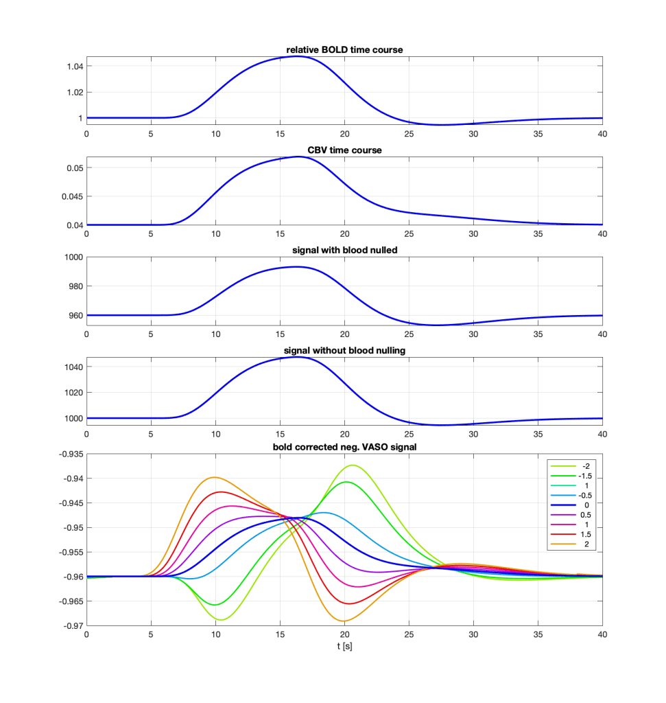
Here I first simulated nulled and not-nulled data assuming a CBV and BOLD response to 10s of activation and subsequent BOLD correction using various misalignments.

One can see in the first figure, that misalignments have an effect on the shape of the estimated VASO response (each color corresponds to a misalignment of the not-nulled signal according to the corresponding number in the legend in seconds before doing the bold correction division). Subjectively I would say that already 0.5 s have a small but possibly relevant effect and that 1 s can change the time-course considerably.

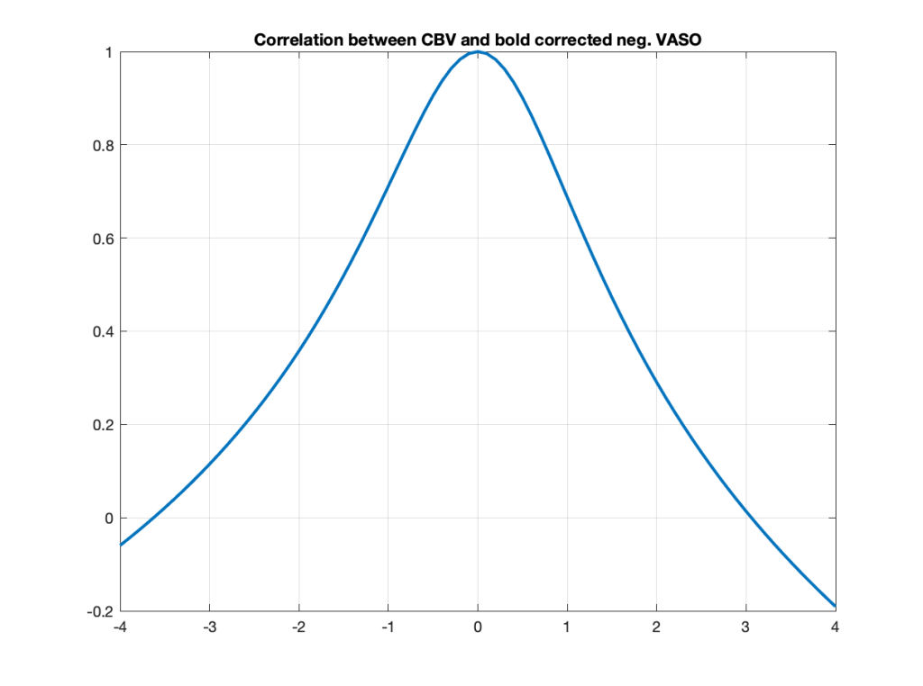
The second figure shows how the correlation between the CBV time course and the estimated VASO time course drops as a function of misalignment before the VASO correction.

3.3 What is the empirical effect of varying the alignment between nulled and no-nulled volumes? – Denis Chaimow

Here I analyzed some data from a flickering checkerboard and finger tapping paradigm of 16s on 16s off, repeated 10 times (flickering and tapping in parallel). I averaged several runs of the same paradigm (in which I varied the Tx voltage, but the results of individual runs seemed to be similar enough).

I first analyzed the BOLD part (not-nulled) using a GLM and defined a voxel mask for all voxels with t-values > 5.

Next I BOLD corrected the nulled volumes by first applying varying temporal shifts (using fsl slicetimer) and then analyzed the resulting VASO data using a GLM with a CBV specific HRF (i.e. no undershoot).

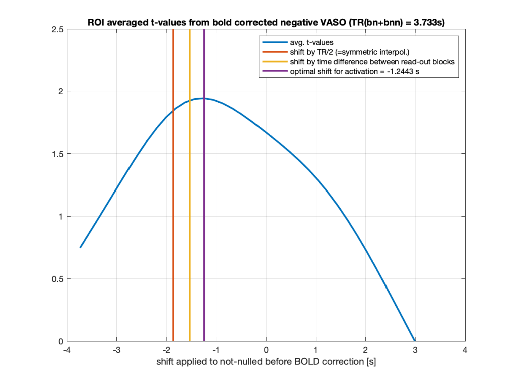
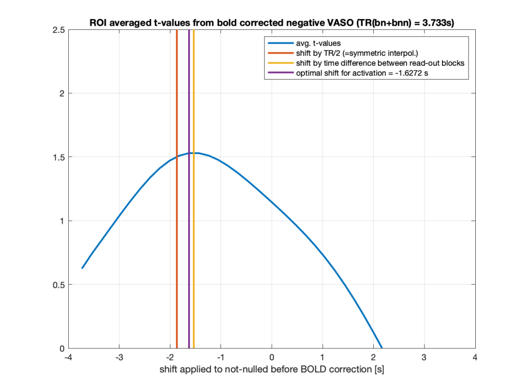
The first figures (datasets from two different subjects) show the average t-values over the previously defined voxel mask for different shifts. It seems that the optimal shift falls relatively close to the time difference between both read-out blocks. However, there does not seem to be a big difference for +-0.5s differences in shift. But larger differences in the shift seem to affect the results.

We can also look at the corresponding activation maps. Here it is difficult to see big differences for +-1s, but we do get less activation for larger deviations from the optimal shift.

3.4 Empirically re-tested effects of temporal shift on the effectiveness of the BOLD correction – Renzo Huber

I followed the “standard” VASO pipeline of temporally upsampling of both contrasts (nulled and not nulled). This upsampling was done with 7^th splines via AFNI. It was upsampled by a factor of 2, assuming equi-distant upsampled TRs. This upsampling also included the first image to be duplicated for the nulled contrast and the last image of BOLD to be duplicated to have both nii-timeseries with the same starting time. 

Link to the data is here.

In agreement with Denis’ reasoning that the early weighting of the T1-contrast in VASO is independent of the instantaneous BOLD contamination matches with the peak z-score:

The maximum VASO z-score is achieved for slightly earlier BOLD.

Strangely enough, the peak z-score for BOLD is also better for shifted time courses, this might be due to the temporal mismatch of the trigger compared to the k-space center. 

To get a more intuitive picture of the corresponding time courses, they look as follows: 

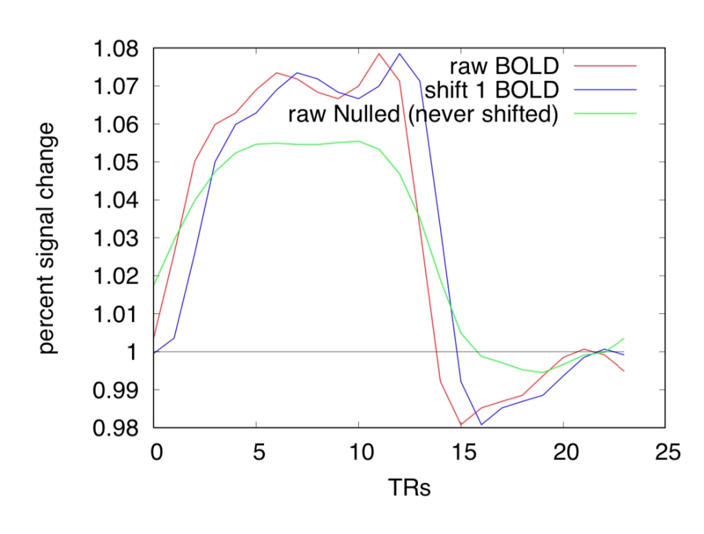
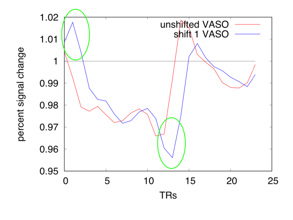
Note that the “optimal” VASO time course that provides the largest z-scores, has strange “horns” at the transients (ellipses). This possibly comes from a BOLD-overcorrection (BOLD contamination that is negatively weighted in the denominator).

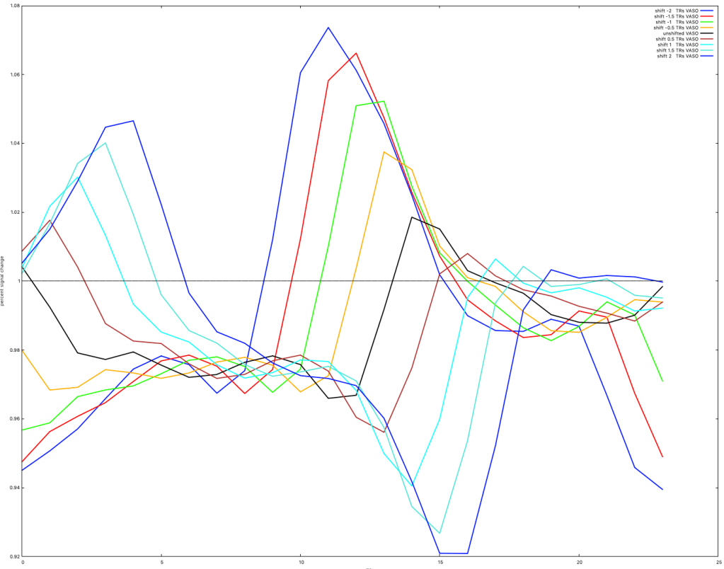
VASO time courses with a large spectrum of shifts applied. Which one does represent the most reasonable looking time course? The transient-horns are getting stronger for larger shifts. 

3.4 Empirical investigation of temporal shifts in another dataset – Sebastian Dresbach

The effect of temporal alignment of nulled and not-nulled images was further investigated in another VASO dataset looking at the sensorimotor system. A jupyter notebook can be found here.

4. Does it matter at what stage BOLD correction is done?

The BOLD correction divides one typically noisy image by another typically noisy image. It may seem intuitive that this could be problematic and that a better approach is to first proceed with all analysis stages that might reduce the noise level such as run averaging, trial averaging or possibly some kind of response estimation before applying the BOLD correction. Is this intuition correct?

Below, we briefly discuss this. We find that it generally should not matter too much if the tSNR is not incredibly low (tSNR < 10).

We can consider a nulled and not-nulled data value to be samples from two normal distributions, where their means m_bn and m_bnn represent the signal and their approximately equal standard deviations σ represent the noise level.

The ratio of the two random variable can under certain conditions (which mainly depend on the coefficients of variation being small enough and which I believe are met in this case) be approximated by a normal distribution with standard deviation σ_VASO given by:

Subsequent averaging by a factor of N would reduce this variance to:

Both transformations show direct proportionality to their respective “input” variances. It is therefore evident that the order of transformations – bold correction and averaging – should have little effect on the variance of the final estimate.

The assumption of 

In this case,

is true in most cases.

In cases, where the tSNR is extremely low, however, a small noise amplification can be expected: 

• For a tSNR of 20, the noise amplification is in the range of 2-3%.
• For a tSNR of 15, the noise amplification is in the range of 5%.
• For a tSNR of 10, the noise amplification reduces the tSNR by about 15%.

Other tSNR values can be quickly simulated by means of a google spreadsheet with random numbers here.