The MP2RAGE sequence is very popular for 7T anatomical imaging and is very commonly used to acquire 0.7-1 mm resolution whole brain anatomical reference data. Aside of this common application, it can also be very helpful for layer-fMRI studies to obtain even higher resolution T1 maps in the range of 0.5mm iso. However, when optimizing MP2RAGE sequence parameters for layer-fMRI studies, there are a few things that might be helpful to keep in mind.

In this post, I would like to discuss the challenges of using the popular MP2RAGE sequence in layer-fMRI studies. Specifically I will discuss challenges/features regarding:

• Background noise.
• Foldover artifact at very high resolutions.
• Usage of double-partial Fourier imaging.
• Inflow into arterial vessels.

Background noise

One of the big advantages of the MP2RAGE sequence is that it is (virtually) free of biases from B₁, or T₂ ^* and provides a ‘clean’ and quantitative T₁ contrast. This is achieved by combining two individual images that are acquired at different inversion times in the form of a complex-valued division. This division, however, may result in some unwanted noise amplification in the background (dividing zero by zero).

For most applications of MP2RAGE, this is not a big problem. In most cases, the noise amplification is confined to locations outside the brain, where we are not interested in the signal anyway. In some layer-fMRI applications, however, this noise amplification can be a challenge.

In layer-fMRI, it is common to use very high-resolution anatomical reference data with resolutions in the range of isotropic 0.35-0.6 mm. Since it would 30-60 min to acquire a whole brain dataset at this resolutions, it is customary to acquire a local slab of the high-res data only. With appropriate GRAPPA acceleration, such a high-resolution slab can be acquired in 2-4 min. For high SNR, however, it is helpful to acquire 2-3 repetitions of such a slab and retrospectively align them and averaged them together. The big challenge of the noise amplification in non-brain areas is that the alignment algorithms can be affected by the background noise and do not perform with their best accuracy. Thus, it can be helpful to suppress the background noise with an additional regularization term during the complex division.

This approach was originally developed from Kieran O’Brian in order to improve the accuracy of segmentation algorithms. (In case you have an ISMRM account you can watch the video of Kieran O’Brian here).

For the newer MP2RAGE WIP sequences, this regularization term can be adjusted in the sequence special card as lambda. In case you do not have the newest WIP version, or you want to optimize the noise removal retrospectively, you can use the implementation in LAYNII as follows:

LN_MP2RAGE_DNOISE -INV1 INV1.nii -INV2 INV2.nii -UNI UNI.nii -beta 0.2

In case you prefer Matlab code for the denoising, Jose Marques also has a Matlab version of it on his Github.

This background removal algorithm can also be quite nifty in VASO layer-fMRI.

Foldover at slab data

Almost all layer-fMRI studies are focusing on specific cortical areas only and do not require whole brain coverage. Thus, there is no need to acquire the high-resolution anatomical reference data for the whole brain either. This would result in impractically long acquisition times. Instead, it is beneficial to use a slab-selective 3D-acquisition approach. With the default parameters of the SIEMENS MP2RAGE sequence, however, this can result in severe fold-over artifacts that render up to 45% of the slices unusable (see gif animations below).

With a bit of tweaking and almost no hit in SNR, the usable number of slices can be substantially increased.

The default excitation pulse of the SIEMENS MP2RAGE sequence has a Bandwidth-Time-Product (BWTP) of 6.4. Which means that the excitation profile is not super sharp. By changing the RF-mode in the sequence special card from Fast to Normal, the BWTP is doubled to 12.7.

The only (negligible) drawback is that the SAR inceases by 0.5-1.5% and that the minimal TR increases by 1 ms. Pushing the BWTP even further to 25, would reduce the fold over artifact even further (shown in fig below).

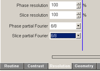
Usage of double partial Fourier imaging

Most 3D-sequences allow partial Fourier imaging in either one of the two phase encoding directions. This is also the case for the SIEMENS MP2RAGE sequence. This allows to user to have the maximal flexibility to optimizing the sequence parameters. As such, dependent on the application, it can be beneficial to apply partial Fourier imaging in one specific direction only. E.g. for the Multi-echo MP2RAGE, when the readout blocks are long and the total number of TRs is not critical, it can be beneficial to apply partial fourier in the first phase encoding direction. Whereas, for another application, E.g. when the readouts are already short enough (e.g. for small matrix sizes) but the acquisition time should be reduced, it is beneficial to apply partial Fourier imaging in the segment (partition) direction.

There is a common misconception about partial Fourier imaging. Namely that partial Fourier could be applied in both direction simultaneously. This is not the case! Only because the protocol editor allows you to do this, does not mean that it is a good idea.

The Hermitesch property of k-space that is employed for partial Fourier imaging (Feinberg 1986) is based on a point-symmetry of k-space F*(k) = F(-k). This property however, refers to the entire k-space vector k and cannot be transferred to any arbitrary direction F*(k_x, k_y) ≠ F(-k_x,k_y) and F*(k_x, k_y) ≠ F(k_x,-k_y). Thus, the outer k-space lines that are representing the high spatial resolutions cannot be recovered in all directions.

Thus, applying partial Fourier imaging in both directions is like resampling low-resolution data to a voxel grid that that is finer than the acquire k-space allows.

This means that in the diagonal direction the effective resolution can be considerably lower than in the other directions.

For partial Fourier imaging of 5/8 and 5/8, the effective resolution in the diagonal direction would be reduced to 28%. This means that a nominal resolution of 0.7 mm would in fact be 2.5 mm, instead! Through k-space zero-filling, this resolution would just be resampled (interpolated) to a 0.7 mm voxel grid.

For partial Fourier imaging of 6/8 and 6/8, the effective resolution in the diagonal direction would be reduced to 35%. This means that a nominal resolution of 0.7 mm would in fact be 2.0 mm, instead! Through k-space zero-filling, this resolution is just resampled (interpolated) to a 0.7 mm voxel grid.

For the use of layer-fMRI, it can be very valuable to obtain high resolution reference data, where the effective resolution is the same across all directions. Thus, I would highly recommend not to to use PF imaging in two directions at the same time. If you don’t have the time to do acquire the entire k-space in at least one phase encoding direction, I would suggest that it makes more sense to lower the matrix size and reduce the nominal resolution in the first place. In this way, the resolution reduction will as least be the same in all directions.

Inflow into arterial vessels.

For 3D-readouts in the MP2RAGE sequence, the inversion pulse is sought to be “global”. However, for layer-fMRI applications, we usually need 7T field strengths with “local” RF coils available only. This means, that in the best case scenario, the inversion pulse is played out with a head-only transmit coil. And it can happen that fresh (non-inverted) blood that was outside the coverage of the transmit coil during the time of inversion has flown into the imaging region during the readout modules of the sequence. This inflowing blood is not inverted and mimics magnetization components that would have been already fully decayed back to equilibrium with very short T1 relaxation times. Thus, dependent on the exact choice of the inversion times, there can be very bright voxels at the location of the arterial vessels. This effect has been described in the some of the first human 7T studies and can even be used for vessel segmentation.

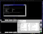
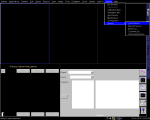
Appendix: How to look at k-space at the scanner

If you want to look at raw k-space data and in case you don’t want to deal with exporting twix filed offline and extract individual coil data on your own, you can also look at k-space data directly at the scanner console. Here, I try to describe a click sequence to do so.

T1 estimation

On the new SIEMENS Syngo platform VE (e.g. the Terra). One needs a license to convert the UNI image to a T1 map. This can be in the form of the MapIt or the WIP925B (from Tobias Kober). There are two work-arrounds.

1.  Off-line processing with Matlab tools from Jose Marques: https://github.com/JosePMarques/MP2RAGE-related-scripts.
2. Retro-recon at the scanner with the following steps.

Acknowledgement:

All LAYNII program executions are tested for version v.1.5.6 and will probably work for later versions too.

I thank Faruk Gulban for discussions about the inflow artifact. I want to thank Ben Poser for help with the excitation pulse BWTP. I thank Sri Kashyap for discussions about the MP2RAGE denoising.