Doing layer-fMRI sometimes feels like doing nothing more than noise management. One must have a full grown masochistic personality trait to enjoy working with such messy data. Namely, layer-fMRI time series data suffer from each and every one of the artifacts in conventional fMRI; they are just much worse and there are also a few extra artifacts that we need to worry about. As such, layer-fMRI time series usually suffer from amplified ghosting, time-variable intermittent ghosting, non-gaussian noise, noise-coupling, motion artifacts, and signal blurring.
Thus, we need to have a set of metrics that tell us whether or not we can trust our specific data sets. We would like to have quality assessment (QA) tools that tell us when we need to stop wasting our time on artifact-infested data and throw them away. It would be extremely helpful to have tools that extract a basic set of QA metrics that are specifically optimized and suited for sub-millimeter resolution fMRI artifacts.
This blog post discusses a number of these layer-fMRI specific QA metrics and describes how to generate them in LAYNII.
Conventional fMRI QA is not applicable and not sufficient for layer-fMRI
Rigorous quality assessment of fMRI time series has become a fundamental pillar of any good code of conduct in fMRI research. In conventional fMRI, a consensus about good practices has been found and these practices are implemented in the major standardized analysis streams. Including QA metrics of 1.) temporal signal to noise ratio (tSNR), 2.) head motion displacement estimates, and 3.) variance explained by ‘neural’ components in ICA. However, in layer-fMRI, these QA metrics are not sufficient. Sometimes they are even completely inapplicable.
- tSNR is not a good measure to capture artifact-induced variances in thermal noise dominated layer-fMRI data. tSNR is calculated as the ratio of the mean signal divided by its standard deviation (STDEV). The crux in this way of estimating tSNR is that the standard deviation usually consists of multiple sources of variance that non-linearly add on top of each other.

tSNR maps with deliberately bad shim. Here the flip angle is lowered. This reduces the signal as well as signal dependent artifacts, while maintaining the thermal noise. The larger relative thermal noise component ‘hides’ the signal-dependent intermittent ghosting due to non-linear variance interaction. As shown in the figure above, for thermal noise-dominated data, fMRI artifacts are not well captured in tSNR maps.
(Note that the reasoning in the figure is not to be misunderstood that tSNR is an inadequate metric for estimating the relative signal stability. It indeed is adequate for overall stability quantification. However, it is not well suited to investigate relative stability losses (changes) in presence of thermal noise.
- Motion traces are not sufficient to assess the data quality. All fMRI protocols are affected by head motion. Thus, it has become standard procedure to manually check the displacement estimates. While this is critically important for layer-fMRI too, it is not sufficient. In layer-fMRI motion usually comes along with higher-order problems too. Namely, even when the rigid head motion can be corrected for, motion-related distortion changes and motion related B0-changes cause intermittent artifacts.

Motion in layer-fMRI is problematic beyond the displacement estimates. It can be seen that due to the low bandwidth that is necessary at sub-millimeter voxels, motion can result in time-varying shading patterns. Strong shading can already sometimes be present with 1 mm displacement, while in other cases, 2 mm motion can be corrected without strong artifacts. For rigorous quality assessment of layer-dependent fMRI data, more appropriate QA metrics are needed.
-
Variance explained by ‘neural’ components in ICA. This fMRI data quality metric received a lot of attention in the last decade. To calculate this metric, the fMRI data are separated with an independent component analysis (ICA). The individual maps are then categorized to be either ‘neural’ or ‘non-neural’ (e.g. artifacts). Ultimately the number of neural components compared to non-neural components and their respective variance explained, is calculated. While this approach has been very useful for finding the optimal acceleration parameters in the HCP study and it has been helpful to find the optimal sequence setups in Multi-Echo EPI, it is not really suitable to judge the quality of layer-fMRI data.
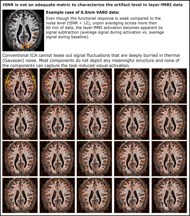
Even though, ICA has an amazing ability to separate components that are associated with non-Gaussian noise, ICA does not work very well when the desired signal is hidden below a huge Gaussian noise floor. It requires a minimum SNR to work robustly and it requires a relatively strong sources of signal fluctuations compared to the Gaussian noise floor. These conditions are not fulfilled for layer-fMRI.
Since the above discussed conventional QA metrics are limited in layer-fMRI data, additional metrics are needed. This blog post, tries to advocate a few candidates of alternative QA metrics and it shows how to generate them in LAYNII.
Layer-fMRI relevant QA metrics from time course analyses on a voxel-by-voxel level

There are a number of established QA metrics established that aim to combine an entire time series into one single value for every voxel. Such measures are very useful as they can be summarized in 3D-signal maps. The most common used parameters that are usually being looked at, for every run in every session, are:
- Mean: The mean is often used as a zeroth order artifact detection tool and it has the highest quality requirements (figure above).
- tSNR: The tSNR is mostly used as a first order artifact detection tool. The higher the tSNR, the better the data quality. It is not considered to be a huge problem, if the tSNR is spatially inhomogeneous. I.e. when there are individual areas with lower tSNR compared to other areas, researchers are usually not alarmed as long as the overall tSNR is not too low. Regional variances are expected for multiple reasons including: RF-coil proximity, large vessels, B0-voids etc. As discussed above, tSNR is not well suited to capture layer-fMRI artifacts.
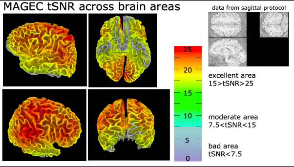
Typical tSNR variations across the brain. Example from 0.8mm whole brain MAGEC-VASO data. - Activation scores: In layer-fMRI publications, activation z-score maps or t-score maps are often shown to support claims about high signal quality. For a good data set, the activation scores are desired to be high in the area of interest, without false positives in voxels that are believed to be unaffected from the task (CSF, GM, unrelated GM).
Beyond these zeroth and first order QA measure maps, there are a few useful higher-order QA metrics that are becoming more and more popular in layer-fMRI method studies. These measures are related to the specific challenges of layer-fMRI acquisition methods. As such, sub-millimeter fMRI data are mostly acquired with EPI sequences with large matrix sizes. Due to the large k-space, the gradients are usually pushed to their respective limits, which comes along with eddy-current artifacts and phase-errors. Furthermore, layer-fMRI can usually only be acquired with relatively low bandwidths and at high magnetic field strengths. Both factors amplify susceptibility-induced image artifacts and intermittent ghosting.
These artifacts are usually not very clearly visible in zeroth and first order QA metrics like mean and tSNR. Higher-order QA measures, however, can capture these artifacts and make them apparent as well.
- Kurtosis and skew: Since, most layer-fMRI data are mostly being acquired in the thermal noise dominated regime, the noise can often be considered to be Gaussian. This means that non-thermal noise (e.g. artifact-induced noise) can be identified by its non-Gaussian characteristics. Two useful measures to quantify how non-Gaussian a noise distribution is, are the measured by means of kurtosis and skewness.
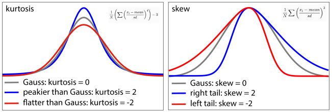
In my own data, EPI ghosting, GRAPPA ghosting and phase-errors in segmented EPI acquisitions usually result in holes of very low (negative) kurtosis values. The respective skewness is then either more positive than usual or more negative than usual.

I want to thank Avery Berman for referring me to the skewness measure in his 2019 ISMRM abstract.
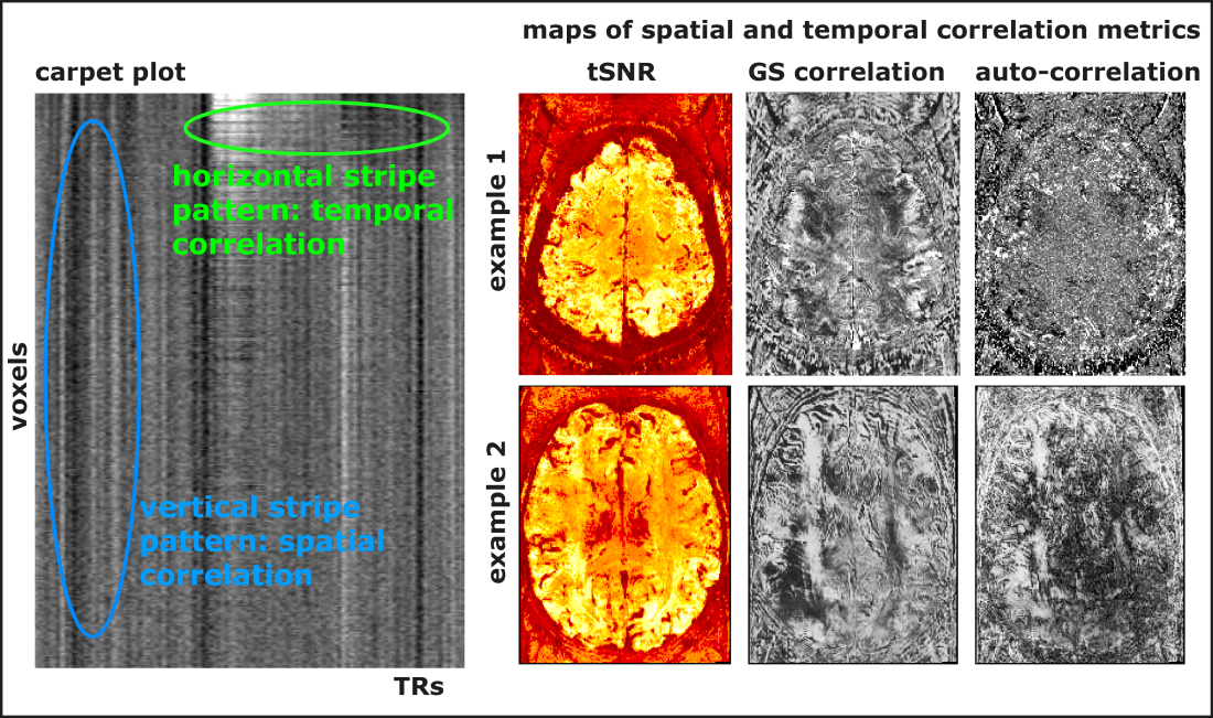
- Auto-correlation and correlation with global signal. While thermal noise is not coupled across space and time, some forms of layer-fMRI artifacts result in strong noise coupling. This noise coupling can be used to filter out artifacts and depict them despite the presence of Gaussian noise. Such spatial noise coupling or temporal noise coupling has often been used to detect artifacts. One popular artifact detection tool is using so called carpet plots (E.g. as done in 3dGrayplot in AFNI). In these carpet plots, every voxel’s time course variations are plotted next to each other (figure below). This allows the researcher to investigate whether there are temporal or spatial correlations visible as horizontal or vertical patterns. While these carpet plots are very useful, they do not really provide a very intuitive idea about where the respective artifacts are coming from. Thus, it can be advantageous to collapse the temporal or spatial correlation patterns onto voxel-wise maps by means of autocorrelation and global signal correlation measures.
Auto-correlation values describe how well the signal at a given point in time can predict the signal at the following point in time. I.e. it has high values when consecutive time points are coupled, which refers to horizontal lines in carpet plots. This could be indicative of slow intermittent ghosting or frequency/phase offset drifts.
The correlation with the global signal describes how much each voxel is responsible for vertical lines in the carpet plot. I.e. it has high values when the signal in any given voxel represents the overall signal fluctuations. Common artifacts that I often see in these maps are related to head motion or temporal GRAPPA interference patterns.
While both of these QA metrics (auto-correlation and GS-correlation) are useful tools for artifact detection, it is important to keep in mind that they also contain non-artifact signals too. E.g. for large scale functional tasks like respiration challenges or vigilance paradigms, these QA metrics might be dominated by task related effects too.
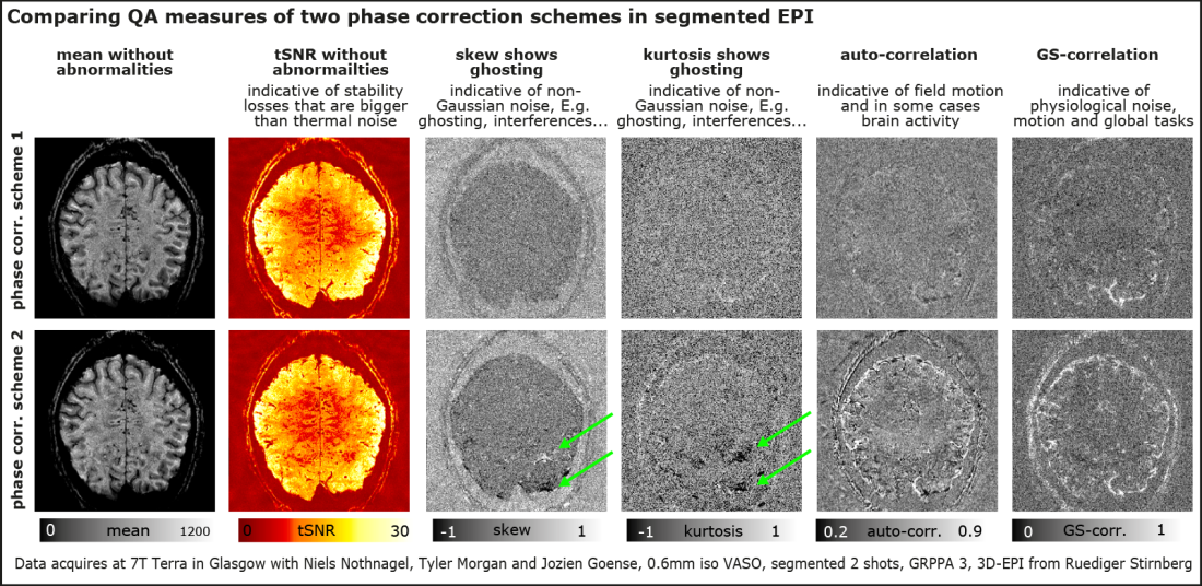
Example application of using higher-order QA metrics to find optimal sequence parameters.
As an illustrative application example of higher-order QA metrics is shown in the figure below. In this pilot study, it was desired to determine which of two potential phase corrections schemes works better 1.) using a global phase correction for the entire time series, or 2.) using a TR-specific phase correction approach. Since the corresponding intermittent ghosts are smaller than the thermal noise, both approaches resulted in very similar mean and tSNR maps. The skew and kurtosis maps, however, can capture the corresponding non-Gaussian noise and make the artifacts more apparent. Similarly, the autocorrelation can capture some of the instability that comes along with the inaccurately updated global frequency, which can become visible as motion and elevated noise level at edges. Thus, by means of these higher order QA metrics, it was possible to make an informed decision about which phase correction scheme to use in further experiments: Scheme 1.
For another application example of using higher order QA estimates, see Avery Bermans 2019 ISMRM abstract.
Generating QA measures in LAYNII
The LAYNII software suite comes along with an example data set (in the test_data folder on Github), which can be used to test the estimation of the above discussed QA metrics. E.g., one can generate an example of all the above discussed QA maps for the time series lo_BOLD_intemp.nii with the following command:
../LN_SKEW -input lo_Nulled_intemp.nii
This command writes out the entire collection of QA metrics: mean, tSNR, skew, kurtosis, auto-correlation, and the correlation with the global signal.
Note, that some of the above described QA measures can also be derived in alternative software suites. E.g. AFNIs 3dTstat can be used to estimate the Mean, tSNR and auto-correlation maps too.
Noise coupling and signal-blurring
While the above QA metrics are very useful to characterize the time course quality of individual voxels, they cannot easily capture spatio-temporal interactions. E.g. if neighboring voxels share the same sources of noise (e.g. due to spatial signal leakage), the above mentioned QA metrics are ignorant to this. This is particularly problematic because in layer-fMRI, the EPI readout is usually very long and, thus, it is expected that the corresponding layer-fMRI data are suffering from unwanted temporal noise coupling between neighboring voxels.
In order to characterize the strengths and the pattern of the temporal correlation of neighboring voxels, a so-called noise kernel calculation is implemented in LAYNII as described below.
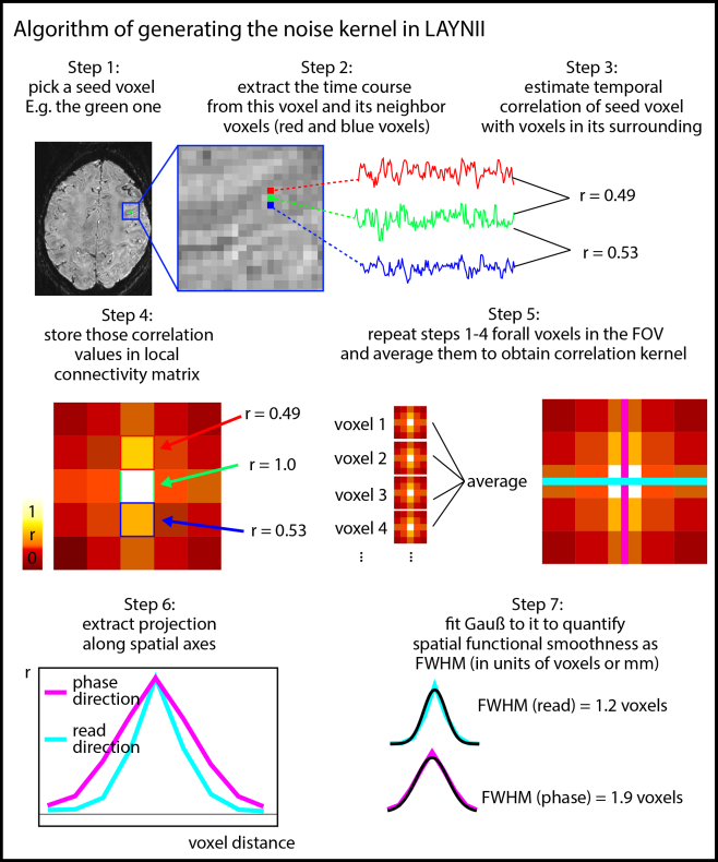
The LN_NOISE_KERNEL program basically estimates the average temporal correlation of neighboring voxels. In contrast to functional smoothness estimations in alternative software suites, LN_NOISE_KERNEL does not simplify the noise coupling with one single FWHM value. Instead it also writes out the 3-dimensional noise kernel as a nii file. This can be advantageous compared to summarizing FWHM values in multiple aspects: As opposed to a single FWHM value, a full noise kernel can capture negative side lobes, anti-correlations, as well as common saw-tooth patterns between odd and even lines. Furthermore, it also provides estimates along the diagonal directions, which can be helpful for 3D acquisition sequences (3D-EPI or 3D-GRASE).
Application examples of LAYNIIs noise kernel
- Estimating the effect of T2*-relaxation: In layer-fMRI EPI with large matrix sizes, the readout duration is usually in the range of the T2*-decay rate, this can result in signal leakage along the phase encoding direction. The noise kernel as described above can characterize how the related noise coupling is affected in the phase encoding direction compared to the read/slice direction. This T2*-blurring is particularly strong in center-out k-space trajectories, e.g., in spiral EPI acquisitions (see example in figure below).
- Estimating the effect of T1-relaxation: In non-BOLD layer-fMRI acquisitions (e.g. VASO or ASL) the readout window is usually following some sort of T1-preparation module. The respective T1-signal buildup during a 3D signal acquisition can result in negative signal leakage (anti-correlation) and edge-enhancement effects. This form of T1-related image sharpening can be empirically investigated by means of the noise kernel.
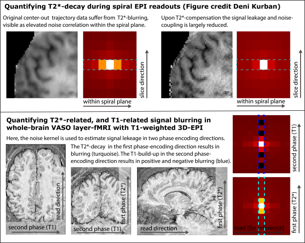
Example applications of the noise kernel to characterize signal leakage along different directions. The top row refers to estimating T2*-related blurring in spiral readouts (see study from Deni Kurban, OHBM 2020). The second row refers to a whole brain VASO protocol with different signal leakage in different phase encoding directions of a long 3D-EPI readout.
Limitations of the noise kernel as a measure of functional localization specificity
- It is to note that data sets with a large imaging coverage might not be well characterized by one single noise kernel only. E.g. it can happen that some brain areas or tissue types with shorter T2*-decay rates will have more signal blurring than other brain areas or tissue types with longer T2*-decay rates. And thus, the respective noise kernel can be area-specific and tissue-type-specific. If the program LN_NOISE_KERNEL is applied to all voxels (default behavior), an average noise kernel of all areas and tissue types is generated. If specific areas are of interest only, an additional mask needs to be provided to estimate the noise kernel with this area only.
- The noise kernel is not a good measure for absolute localization specificity quantification across different SNR-levels. As such, when a time series has more random noise, each voxel’s time course looks uncoupled from its neighbors. This would be even the case when the fMRI signal below the noise floor would be highly coupled and, thus, the resulting noise kernel would falsely suggest a high localization specificity. This means the sharpness of the noise kernel should only be interpreted with respect to a reference (e.g. read-direction, control scan).
- It should not be assumed that temporal correlation of neighboring voxels must solely come from artifacts. There might also be neural or physiological reasons for it. Thus, in the above examples of T2* and T1 related noise coupling, it is necessary to have a control condition of the read/slice direction, for comparison.
Example application of generating a noise kernel with LAYNII
The LAYNII software suite comes along with a test data set (in the test_data folder on Github), which can be used to test the application of the LN_NOISE_KERNEL program. E.g., one can generate an example noise-kernel from the example time series file lo_BOLD_intemp.nii in LAYNII’s test_data folder with the following command:
../LN_NOISE_KERNEL -input lo_Nulled_intemp.nii -kernel_size 7
I believe that other software packages use similar algorithms to estimate the functional point spread function for the estimation of statistical algorithms of cluster sizes SMOOTHEST (program in FSL) or 3dFWHMx (in AFNI).
VASO specific quality assessment
While all of the above QS metrics are applicable to any fMRI time series of any sequence and contrast. There are some additional QA metrics that provide additional information for fMRI modalities with multiple contrasts, such as VASO, ASL, Multi-Echo etc. In those modalities, fMRI measures can be calculated by multiple concomitantly acquired time series. Since VASO is particularly suited for layer-fMRI, the below examples will focus on VASO only, while the QA metrics are applicable to other multi-contrast data too.
BOLD-VASO synchronicity
In virtually all layer-fMRI applications of VASO, the sequence acquires BOLD reference images concomitantly. This means that the different contrasts can be investigated with respect to synchronous and anti-synchronous fluctuations. If there are fluctuations that are synchronized and in phase it usually refers to neural activity, if there is a bit of a temporal delay it refers to big vessels, and if there are fluctuations that are synchronized and no anti-correlated it could refer to artifacts. (For more information see this abstract)
Such temporal voxel-wise correlations of two simultaneously acquired time series can be generated with and without variable temporal lags in the LAYNII programs LN_BOCO, or LN_CORREL2FILES.
Example application of generating a synchronicity metrics with LAYNII
LAYNII’s test_data folder on Github contains the example time series lo_BOLD_intemp.nii and lo_Nulled_intemp.nii, which can be used to generate an example of all the above discussed BOLD-VASO interaction maps with the following command:
../LN_BOCO -Nulled lo_Nulled_intemp.nii -BOLD lo_BOLD_intemp.nii -shift -output lo_VASO
../LN_CORREL2FILES -file1 lo_VASO.nii -file2 lo_BOLD_intemp.nii
VASO usually has less artifacts than BOLD
The VASO signal is estimated based on multiple, simultaneously acquired time series. This can have some fortunate effects on the artifact level. As such any slow-varying artifacts that are simultaneously happening in multiple inversion time images, can be canceled out in the resulting VASO signal. Thus, the above discussed QA metrics often look better in VASO compared to single contrast time series.

I do not know why VASO usually provides cleaner maps of higher order QA metrics. It is probably a combination of multiple factors.
- a) Due to the lower tSNR in VASO compared to BOLD, many artifacts are just more hidden under the higher thermal noise level.
- b.) The dynamic division of image signals with and without blood nulling does not only correct for BOLD contaminations, but also other unwanted signal contributions. As such, slow signal drifts and slow phase error-related ghosts are inherently corrected for in VASO.
Acknowledgements
I thank Avery Berman for the suggestion of using the skew as a measure of intermittent ghost level as described in his 2019 ISMRM abstract. I want to thank Deni Kurban for sharing her center-out spiral VASO data as an example of the noise kernel estimation. I want to thank Nils Nothnagel, Tyler Morgan and Jozien Goense for acquiring the data that are shown in the gif animation about motion-induced shading artifacts. I thank Eli Merriam for suggesting the BOLD-VASO correlation maps as a function of time shifts as applied in the last section. I would like to thank Faruk Gulban for his contributions to LAYNII (2.0) and documentations in LN_BOCO, LN_SKEW and LN_CORREL2FILES.
All program executions are tested for LAYNII version v.1.5.6 and will probably work for later versions too.
