Quick example of cortical unfolding in LAYNII

Update June 2021: There is a new and more comprehensive 3D-supported LayNii Program for cortical unfolding. Please see https://thingsonthings.org/ln2_multilaterate/

The blog post below is kept for archiving purposes: 

In this Blog post, I seek to describe a quick example of how to analyse high-resolution data across layers and columns with LAYNII.

This post is motivated by Shinho Cho. I want to thank Shinho for providing the example data used here. 

There are 5 steps involved to unfold the cortex.

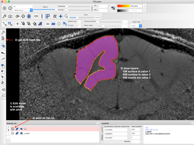
1.) Obtain border lines of GM/WM and CSF.

This can be done with automatic segmentation algorithms or manually in FSLeyes.

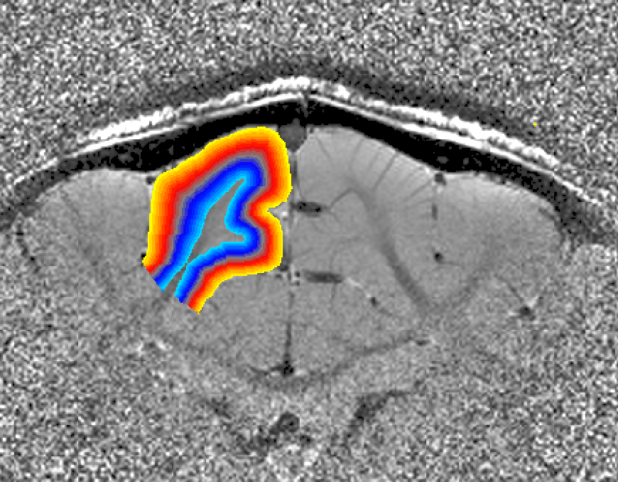
2.) Calculating layers with LN_GROW_LAYERS

With this rim.nii file, LAYNII can generate the layers with the command:

LN_GROW_LAYERS -rim rim.nii -vinc 100

The result is a layer file layers.nii looking like this

Note on single slice data (e.g. for Shinho Cho ): when the “-threeD” flag is not set, the program LN_GROW_LAYERS estimates the layers on a slice-by-slice basis. This is done assuming that the slice direction is the third dimension in the nii header according to the default of x-y-z,as phase-read-slice. If your data are not stored like this, consider using the “-threeD” option in LN_GROW_LAYERS. Alternatively, the dimentsion can be exchanged with fslswapdim input x z y  output.

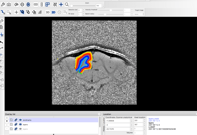
3.) Setting landmarks

For the columnar distance calculation, you can choose a landmark manually anywhere in the layer.nii. E.g generate a new file that is everywhere zero except for one column, where the signal is 1.

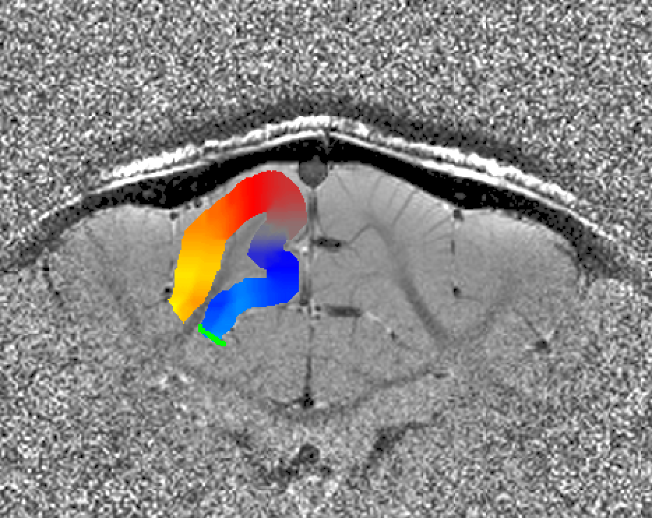
4.) Calculating columnar distances

The columnar distances are calculated in the LAYNII program LN_COLUMNAR_DIST

LN_COLUMNAR_DIST -layer_file layers.nii -landmarks landmarks.nii -vinc 400

Algorithm to estimate columnar distances

The columnar distances are calculated in a 6-step algorithm. The intermediate result after every step can be written out with the “-verbose” flag.

1. The algorithm starts with by estimating Euclidean distances from the manually drawn landmark. In order account for the fact that the GM of a neighboring sulcus can be closer than the distance of a column with in the sulcus, the distance is estimated with a local grow-algorithm that extends the local patch voxel-by-voxel (step-size=1).
   

   

2. Since the growing algorithm works in voxel space, it can only estimate distances in units of intager multiples of voxel distances. The resulting Pythagorus errors can be accounted for with a local smoothing step along the layer direction only.
   

   

3. In the next step, the columnar distances are extrapolated across layers. The columnar distance value of every voxel is simply copied from the next closest voxel that has a valid distance estimate. This is done within the GM ribbon only (to avoid leakage from neighboring sulci). This is by far the longest part of the program. The most superficial and the bottom layers are excluded for now, because it would not be clear which side of the sulcus the correspond to.
   

   

4. Again, this step comes along with some Pythagoras errors that can be accounted for with within-layer smoothing.
   

   

5. Now, the entire rim of the cortex can be filled into pial voxels too. This final growing procedure is only local (in the vicinity of two voxels). Thus, signal leakage of neighboring sulci can be neglected.
   

   

6. In a final step, the user can choose how big the columns should be. This is done with the optional “-Ncolumns” flag.
   

   

Underlying assumptions in this procedure:

• The proposed algorithm only works properly, if the voxel distance is much much smaller than the spatial scale of the curvature.
• The proposed algorithm only works properly, if the voxel distance is much much smaller than the spatial scale at which the cortical thickness changes.
• If the cortical curvature radius is in the range of the cortical thickness, columns thicknesses are scaled accordingly. The middle cortical layer are defined to have a homogeneous distance.
  

  

   

• When the end of the growing area is right as the position, where the curvature radius is smaller than the cortical thickness, this error can be propagated to neighbouring columns. On work around here is to increase the growing area (E.g. using a larger vinc value ).
  

  

5.) Regriding

The layers and distances provide an orthogonal coordinate system that can be used to regrid the data into a 2-dim layer-column matrix.

LN_IMAGIRO -layer_file layers.nii -column_file coordinates_final.nii -data ANAT.nii

The output of IMAGIRO is the file “unfolded*.nii”.

 

Further information on the dataset

Subject: 8 weeks old female cat, Varian 9.4T at CMRR
FOV: 32mm x 32mm, Slice thickness: 0.5mm x 6 coronal slices
Matrix size: 256 x 256, Resolution: 0.125 x 0.125 x 0.5mm, GEMS sequence (T1+T2 weighted), TR/TE = 300ms/15ms
1.5 cm diameter, single loop surface coil (1 channel)

The data shown here can be downloaded here: https://layerfmri.page.link/cat_data

Comment on LAYNII versions

This blog post is written and tested for LAYNII versions v1.0.0 – v1.5.6.

Addendum (Feb 2021)

The program LN_COLUMNAR_DIST used here is aimed for slice-wise definition of columns. For flattening of 3D-patches with that are not aligned in any slice direction, consider using the LN2_MULTILATERATE & LN2_PATCH_FLATTEN approach.