
Authors: Renzo Huber and Faruk Gulban
When you want to analyze functional magnetic resonance imaging (fMRI) signals across cortical depths, you need to know which voxel overlaps with which cortical depth. The relative cortical depth of each voxel is calculated based on the geometry of the proximal cortical gray matter boundaries. One of these boundaries is the inner gray matter boundary which often faces the white matter and the other boundary is the outer gray matter boundary which often faces the cerebrospinal fluid. Once the cortical depth of each voxel is calculated based on the cortical gray matter geometry, corresponding layers can be assigned to cortical depths based on several principles.
One of the fundamental principles used for “assigning layers to cortical depths” (aka layering, layerification) is the equi-volume principle. This layering principle was proposed by Bok in 1929, where he tries to subdivide the cortex across little layer-chunks that have the same volume. I.e. gyri and sulci will exhibit any given layer at a different cortical depth, dependent on the cortical folding and volume sizes (see figure below).
With respect to applying equi-volume principle in layer-fMRI, the equi-volume layering has gone through quite a story. A plot with many parallels to Anakin Skywalker.
In this blog, the equi-volume layering approach is evaluated. Furthermore, it is demonstrated how to use it in LAYNII software.
The chosen one…
In 2010, Marcel Weiss (a PhD Student at the Max Planck Institute CBS, directed by Bob Turner) was reading through the German literature of early brain anatomists. And he found an old book from Siegfried Thomas Bok, a Dutch neurologist. According to Bok, the cortical layers are not always parallel to the cortical surface. But instead, cortical layers seem to move towards the cortical surface at the top of a gyrus and are closer to white matter at the bottom of a sulcus.

Upon Marcel’s (re-)discovery of this equi-volume principle, Miriam Waehnert and her husband Philip were trying to implement the first algorithm for layer-(f)MRI. And with help from Markus Streicher and (importantly) Pierre-Louis Bazin, the first implementation was released as part of CBS-tools. Ever since this algorithm was introduced to the high-resolution MRI community by Waehnert et al., the equi-volume approach was celebrated as the ultimate solution to our layering problems. It was applied in many MRI and fMRI studies and it has been implemented in several softwares e.g., in NIGHRES (previously in CBS-tools), in ODIN, in BrainVoyager, by van Mourik et al, and by Wagstyl et al, and *now* in LAYNII (as of version 1.5.2).
Different results of various layering algorithms in LAYNII.


Unfortunately, however, the application of the equi-volume layering beyond ultra-high resolution (<400-700 micron) ex-vivo samples, can come along with quite a few challenges and limitations. As so often in science, the devil is in the detail.
…that would destroy the noise not join them
In layer-fMRI, every-day life is messy. Data are noisy, the resolution is not as high as we wish it to be, and the biology does not care about our elegant geometrical theories. In almost all layer-fMRI applications, there are some quirks that make me feel uneasy about the equi-volume layering. Below, a few of them are listed.
Equi-volume layering amplifies segmentation noise
While equi-voluming is the most accurate layering approach in high-quality ex-vivo data, it might not be applicable in in-vivo (f)MRI data with limited SNR. Since the equi-voluming amplifies curvature effects following the cortical folding, it also amplifies curvature noise. Consequently, it suffers from segmentation noise, as shown in the example analysis below.

1. Equi-volume layering amplifies discretization noise
In most in-vivo layer-(f)MRI data, the voxel size is not several orders of magnitude smaller than the typical size of cortical folding and cortical thickness. This means that the gray matter borderlines will have some residual level of jaggedness. This form of discretization noise can be misinterpreted by the algorithm as a form of cortical folding and will be amplified in the equi-volume layering.

This effect can be partly accounted for by smoothing the segmentation and/or by incorporating more than one voxel into curvature estimates (e.g. level-sets). However, this comes at the cost of reduced spatial precision of the curvature sampling (see below).
2. Equi-volume layering is a rule about volumes, not layers.
The equi-volume principle dictates that the volume of a layer chunk needs to stay the same, independent of the cortical curvature. However, this rule is ambiguous with respect to how the volume should be defined at a given chunk of cortex. Since a volume is defined by three spatial dimensions, different shapes such as a cube, a cylinder or an ice-cream cone can result in the same volume.
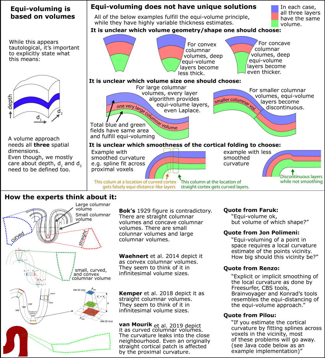
Since the equi-volume layering depends on a definition of a local curvature, it does not necessarily deal very well with abrupt changes of the cortical folding pattern (see figure of empirical data below).

The cyto-architectonic layers in the cortex are always continuous, even at location of abrupt cortical folding pattern changes. This suggests that the biological layers do not *strictly* follow the equi-volume principle and -to some extent- violate it.
3. The equi-volume principle does not seem to fit all brain areas.
The validation of the equi-volume approach has mostly been conducted on very high-resolution data (<250 micron) in small cortical patches of V1. For small patches of V1, the algorithm seems to be more accurate than alternative algorithms.


While the location of the Stria can be nicely predicted in small patches of V1. The results become less clear for larger patches. Namely, there are other reasons why cyto-architectonic layers are not consistently found at a given cortical depth. The curvature bias is just one of many courses of variance.
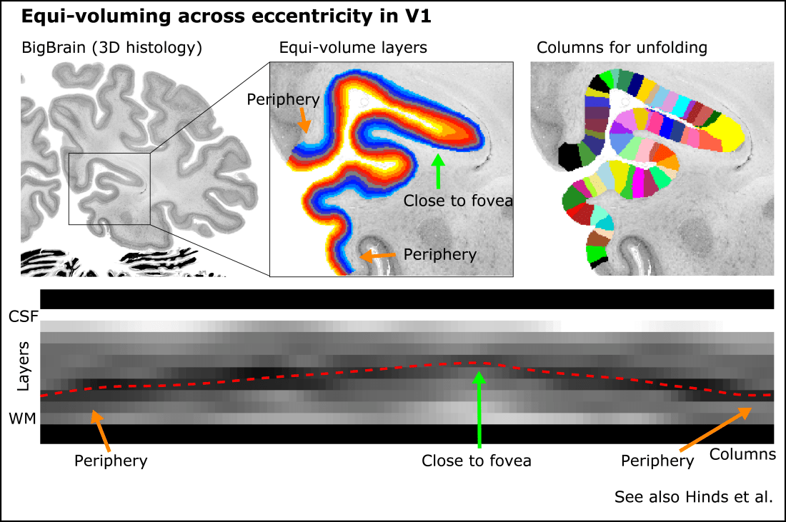
E.g. in the visual cortex, the position of the Stria Gennari is known to be more superficial (closer to cerebrospinal fluid) at the fovea and deeper (closer to white matter) in the periphery (see Sereno et al., 2014, Hinds et al.). Thus, when plotting the layer profiles across a larger patch of V1, the stria Gennari is not a perfect horizontal line.
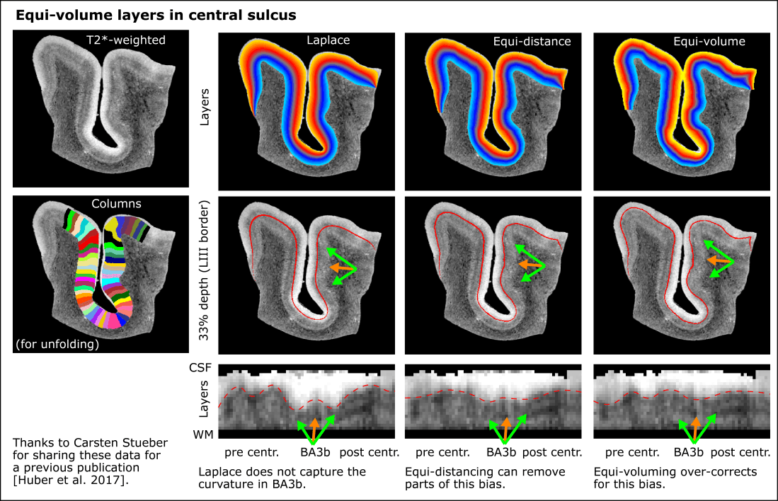
In other brain areas, beyond V1, even the equi-volume algorithm does not seem to work perfectly well. E.g. in the central sulcus, where entire brain areas barely spanning across a few columnar structures, there are sections, where the equi-volume layers amplify the curvature too much and the equi-distant layers seem to be just as accurate.
It might be fixable…
Many of the above limitations of the equi-volume principle can be mitigated to some extent. However, none of those strategies seem to be one-stop solutions.
Smoothing helps
All equi-volume implementations in current software packages seem to be somewhat based on a smoothness assumption. Some implementations explicitly apply smoothing filters on the curvature estimates, while other implementations estimate the curvature based on an assumed smooth local vicinity to begin with. While smoothing of the cortical curvature helps to avoid discontinuous layers, to minimize segmentation noise, and to minimize discretization noise, it results in local inaccuracies of the layer depth.

The cyto-architectonic layers in the cortex are always continuous, even at locations of abrupt local changes of the cortical folding pattern. Hence, the biological cortical layers are inherently smooth to some extent, which might justify the application of implicit or explicit application of spatial smoothing. It is not clear today, however, how the smoothing kernel-size should be chosen. Should it be Gaussian smoothing? Is the smoothing size curvature dependent? Future research is needed to apply the equi-volume principle with the most physiologically plausible algorithm parameters.
Upsampling, vertex analysis and level-sets help to minimize discretization problems
The discretization limitation in the equi-volume approach can be mitigated when the segmentation is defined on a finer spatial grid than the initial resolution. Spatial upsampling, and/or surface analyses using floating point precision vertices can help to mitigate the resulting discretization errors. However, these approaches come along with additional resampling steps and/or much larger file sizes (e.g. up to 50GB per time series).
Since no segmentation algorithm published to date works at a 100% accuracy, every layer-fMRI researcher needs to manually check each dataset for segmentation errors and correct for the biggest ones. This takes approx. 2-8 hours per dataset (and possibly more for whole-brain images). If each dataset would need to be spatially upsampled, the corresponding researchers time investment would become impracticable.
Alternatively, the discretization limitation of the equi-volume principle can be partly accounted for with non-binary level-set analysis and or in vertex-space. In fact, aside of LAYNII, all equi-volume analysis software packages out there use either vertices or level-sets (Freesurfer, Brainvoyager, CBS-tools, Nighres, Wagstyl’s tools and van Mourik’s tools). While those layer-data formats have their benefits in structural whole-brain data, they have certain limitations in the daily practice of layer-fMRI. Vertex-based layer formats and level-set based layer formats are designed for continuous topographically-meaningful, folded surfaces. While the brain technically fulfills these requirements, most layer-fMRI data don’t. In virtually all layer-fMRI data, there are discontinuities, resolution constraints, as well as constraints of brain coverage (commonly 0.5-2.5cm slabs). In these common layer-fMRI data, vertex-based and level-set-based algorithms are only applicable with additional auxiliary data and analysis steps. All of which come along with their own additional challenges.
…but life goes on (with or without it) just as well
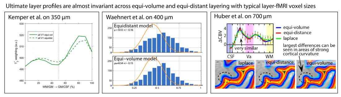
Currently, most layer-fMRI studies use resolutions in the range of 0.7-0.8 mm. At these resolutions, the partial voluming of neighbouring layers in each voxel introduces significantly larger errors than the small difference of equi-volume layers vs. equi-distant layers.
So for now, every researcher should be allowed to decide on their own which algorithm to choose. One has the choice of either dealing with the equi-volume layering limitations mentioned above or having an easier life and using the equi-distant layering with insignificant residual curvature biases. Whatever you chose, the results in practice will be virtually unaffected considering the current image resolutions in layer-fMRI. However, with further development of new imaging sequences (stable multi-shot readouts) and hardware (e.g. Feinbergatron scanner in Berkeley) the effective resolution of layer-fMRI will get higher and higher. Therefore, eventually, we will need to re-evaluate the discussions above.
Equi-voluming in LAYNII
All the discussed algorithms of this blog post are implemented in LAYNII (version 1.5.0 and upwards). You can play around with them, compare them on your own, and test them with the test_data that come along with LAYNII in the test_data folder on github.
In this folder, you can estimate:
Equi-distance and Equi-volume layers with Faruk’s implementation as follows:
../LN2_LAYERS -rim sc_rim.nii -equivol
for the optional application of medium spatial smoothing, use the following flag.
-iter_smooth 50
Equi-distance layers with Renzo’s implementation as follows:
../LN_GROW_LAYERS -rim sc_rim.nii
Laplace-like layers with Renzo’s implementation as follows:
../LN_LEAKY_LAYERS -rim sc_rim.nii
Equi-volume layers with Renzo’s implementation as follows:
LN_GROW_LAYERS -rim sc_rim.nii -N 1000 -vinc 60 -threeD
LN_LEAKY_LAYERS -rim sc_rim.nii -nr_layers 1000 -iterations 100
LN_LOITUMA -equidist sc_rim_layers.nii -leaky sc_rim_leaky_layers.nii -FWHM 1 -nr_layers 10
If you find any issues with LAYNII or want to request a feature, we would be happy to see them posted in our github issues page.
All program executions are tested for LAYNII version v.1.5.6 and will probably work for later versions too.
Acknowledgments
I want to express many thanks Pilou Bazin for inviting me to Amsterdam early 2020 to discuss the discretization challenges. I also wants to thank him for comments on the examples shown in the blue-red-green figure on the columnar volumes. I am thankful to Jonathan Polimeni for explaining me that the equi-volume principle always needs to be based on a local proximity in May 2018. I thank to Carsten Stueber for sharing the M1/S1 ex-vivo sample data. I thank Jozien Goense for sharing the Macaque data. I thank Dimo Ivanov for confirming the history of the early days of the Equi-volume layering. We thank Rainer Goebel for his encouragement and discussions on surface mesh based layering algorithms.
