In this blog post, I want to share my thoughts on the number of layers that should be extracted from any given dataset. I will try to give an overview of how many layers are usually extracted in the field, I’ll describe my personal choices of layer numbers, and I will try to discuss the challenges of layer signal extraction along the way.

It is obvious that the effective resolution in an fMRI dataset cannot be higher than the number of voxels that span across the cortical depth. And it is also clear that any signal variations on a finer scale than the voxel size should not be over interpreted. Thus, I am a bit surprised that the question on the choice of how many layers should be extracted is continuously discussed since many years with great eagerness.

In literally all of the layer-fMRI papers that I co-authored, we were asked by the reviewers why why chose a certain number of layers. And thus, many supplementary materials of our papers contain a section about it. E.g. Fig S6 in Huber 2018, Page e3 of Huber 2017, Page 12 of Huber 2018a. Etc. pp.

How many layers do other researchers in the field extract?

There is really no standard in the field on how many layers should be extracted. (If you disagree, please leave a comment below) In the papers that I usually look at, the number of layers ranges from 2 up to 22 layers.

This slideshow requires JavaScript.

In studies, that chose a number of layers larger than 3, the authors do not assume that the individually extracted layers are statistically independent anymore. I believe the most controversial choices of number of layers are the the ones by Muckli et al., and Kay et al. They chose a number of 6 layers, which is (coincidentally) exactly the number of histologically defined cortical layers, without explicitly assuming that these layers need to match.

Why I personally prefer rather large number of layers

Example data

I would like to discuss my choices of the number of layers below by means of an example dataset. This data set was acquired at NIH in 2017 as part of this study. The data refer to an in-plane resolution of 0.7 mm covering the motor cortex during a 12 min finger tapping task acquired with an 3D-EPI VASO sequence. Data are available for download here. In order to make leakage effected clearer, I generated this pseudo-synthetic dataset. In order to do so, I prepared measured data with several denoising filters and anisotropic smoothing. The ‘raw-data’ input for all analyses done her is depicted in the figure below.

In an ideal case, we want to make these two stripes visible as two individual peaks along a layer profile plot.

So let’s see how the chosen number of extracted layers affects the layer profile of the double stripe dataset.

These data show:

• For very few number of layers (e.g. 2-5), the double peak signature of the data is not really visible in the layer profiles.
• For larger layer numbers (e.g. 10-75), a nice looking smooth double peak can be seen.
• For very large layer numbers (e.g. 100), the profile looks less smooth again.

The shortcomings of choosing too few layers:

In the figure above, it is visible that 20 layers look significantly better than 5 layers. This might be a bit paradoxical at first. Given the resolution and cortical thickness in this example here, there cannot be more than 5 independent voxels across the cortical depth anyway. So how come that it’s beneficial to use more layers than the effective resolution would suggest? I believe that the answer lies in the fact that the layers are not necessarily perfectly aligned with the voxel orientation. Thus, any given layer with a finite thickness pools signal from voxels of a rage of cortical depths.

Based on these considerations it appears that is it beneficial to use many layers, which are considerably thinner than the effective resolution. However, I believe there might be a natural upper limit of the number of layers too and it might not be beneficial to inflate the number of layers too much either.

The shortcomings of choosing too many layers:

When there are more layers than the effective resolution would suggest, the layers must be defined on a finer spatial grid than the voxel size. This means that the data file that defines the layer locations must be larger too.

Since, voxels are volumetric (distance^3) objects, the information content and the file size increases cubily with the up-scaling factor. In my experience, I found that for  conventional fMRI data, the up-scale factors of 2-5 are still manageable. However, for up scale factors of 10 and more, the typical file sizes can be quickly in the the range of several GB and more advanced computing power becomes necessary.

Since the grid resolution is limited by the file size, the number of layers that are to be extracted, must be eventually limited too. As such, when there are more layers calculated than the grid density allows, individual layers can be become sparse, and develope wholes.

My conclusion

For typical 0.75mm datasets, with average cortical thickness of 3-4mm, and slab coverage, I recommend a number of layers that is at least 4 times larger than the effective resolution would suggest. This means that I recommend an up-scaling factors of 4. With typical cortical thicknesses this results in a recommendation of extracting 20 layers.

• When the cortex is thinner (e.g. in V1 or S1), I would recommend to use fewer layers (e.g. 10).
• When the coverage is larger, I would recommend to use less upsampling (e.g. 3) and fewer layers (e.g. 10).
• When voxels are smaller (e.g. 0.5), I would recommend to user more layers (e.g.  40).

Spatial interpolation

In order to work with layer-fMRI data on different grid sizes, we must find a way to transform data across different grid representations back and forth. This transformation can be considered as “interpolation”. Thus, it touches a topic of heated discussions in the field of layer-fMRI, which deserves a blog post on its own.

One of the most feared dangers of spatial interpolations in layer-fMRI is that it might generate features in the final results, that have not been there in the brain.

In the case of extracting layer-fMRI information, I am in favour of interpolation functions of cubic order or higher order. Lower order interpolations can result in ringing artifacts that arise of the sampling voxels of different cortical depth.

This effect has been previously been described by Martin Havlicek in his 2016 OHBM poster.

Extreme case of infinity layers

No matter how many layers we chose to extract, we always end up dividing the cortex into a finite number of bins. If the bins are wider, more voxels contribute to a single bin, which results in larger SNR. However, wider bins also come a long with a reduced effective resolution across depth. If the bins are thinner, less voxels contribute to a single bin, which results in a lower SNR. However, thinner bins also come a long with a higher effective resolution across depth.

It is, of course, also possible to avoid the choice of the layer number all together by omitting the binning step in the analysis. This it effectively the extreme case of choosing an infinite amount of layers, such that every voxel represents it own layer.

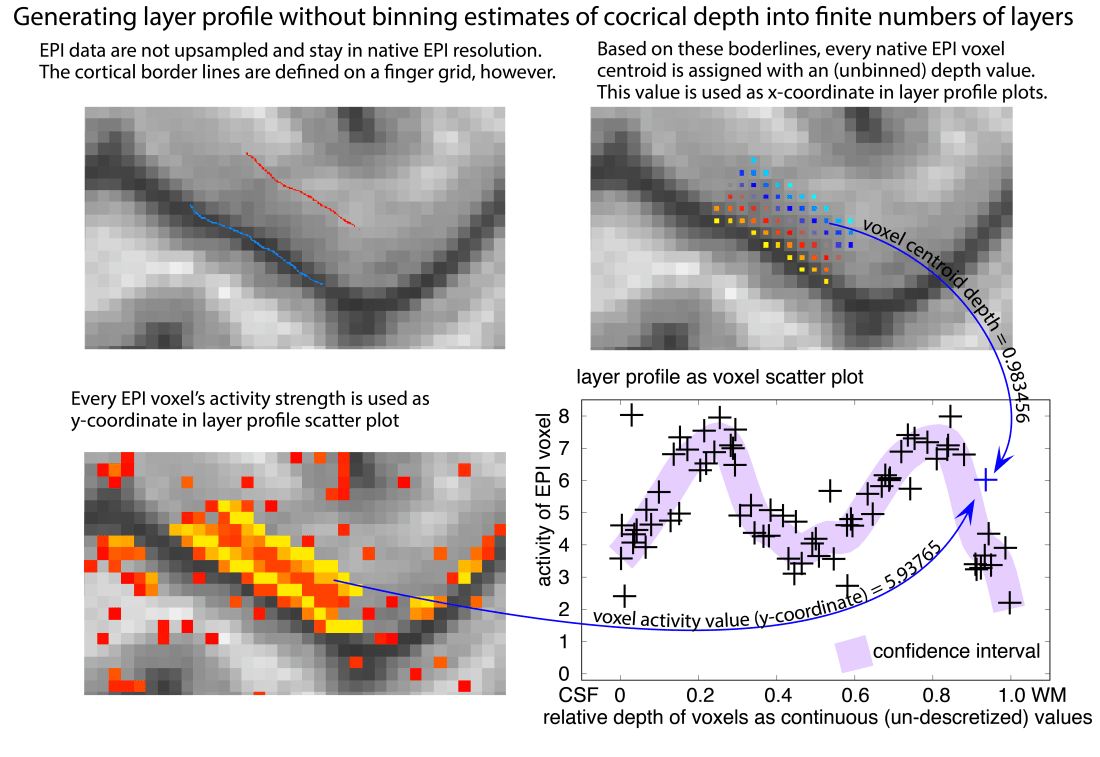
I find this approach particularly nice because it renders any upsampling interpolation unnecessary too. However, in real live data, this approach turns out to be pretty sensitive to noise as it does not allow for averaging across voxels with a similar depth. It is not based on a intracortical coordinate system and hence, it does not allow straightforward cortical unfolding.

Why I do everything in voxel-space

I prefer to conduct layer analyses in voxel space rather than surface space because of the following reasons:

• For new methodologies, such as layer-fMRI analyses, not all potential sources of artifacts are fully understood, just yet. Henc, I find it better to use conservative analysis approaches that keep the analysed data as close to the raw data as possible. This is possible by minimizing number of the analysis steps. Since the original data are acquired in voxel space I, thus prefer to keep them in voxel space as long as possible along the analysis pipeline. This way it is easier to understand the origin of potential acquisition and analysis artifacts in the visualisations of the final results.
• As described from Polimeni, the sampling of fMRI signal in surface space can result in blurring. As such, signal from one voxel can be projected onto multiple layer surfaces. Instead of surface layer extraction, Polimeni proposes to estimate cortical depth in voxel space and sample the information based on the voxel centroid location.

  

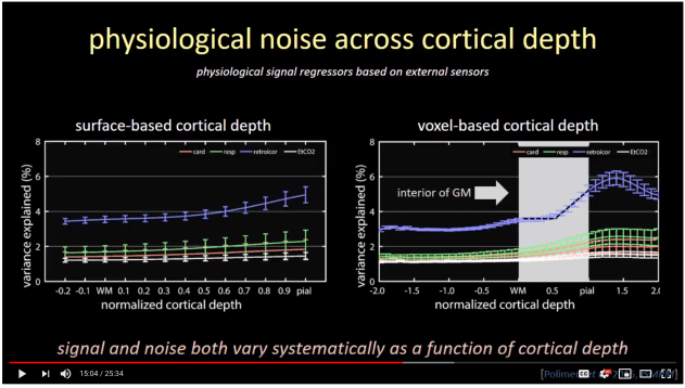
• I happened to be more experienced working with nifti format compared to gii formats. For me, the header information is easier to keep track of, it’s more straight forward in debugging, and the voxel analyses do not require as much computation power compared to surface analyses.
• For surface representations, the information content and the vertex density can be non-homogeneous, which can result in complicated noise coupling effects (Kay 2019)
• Surface representations can come along with strict topological requirements. As such, surfaced often must be closed, without holes. Since there is no practical whole brain layer-fMRI protocol just yet, almost all layer-fMRI data are generated from slab acquisitions and are, thus, naturally not straight forwardly representable by closed surfaces.

Acknowledgements

I thank Martin Havlicek for discussions about depicting the layers as scatter plots. I also want to thank Faruk Gulban for an inspiring talk about related topics and subsequent discussions with him, Ingo Marquardt, and Marian Schneider.