Quick analysis pipeline of getting layer fMRI profiles without anatomical reference data

This is a step-by-step description on how to obtain layer profiles from any high-resolution fMRI dataset. It is based on manual delineated ROIs and does not require the tricky analysis steps including distortion correction, registration to whole brain “anatomical” datasets, or automatic tissue type segmentation. Hence this is a very quick way for a first glance of the freshly acquired data.

The important steps are: 1.) Upscaling, 2.) Manual delineation of GM, 3.) Calculation of cortical depths in ROI, 4.) Extracting functional data based on calculated cortical depths.

1.) finer grid for calculated layers than actual resolution

Here the layering analysis is done on a finer grid than the voxel grid in which the data are actually acquired. This allows the calculation of layers that are smooth and do not depend on the edge angular shape of the voxels. This feature is particularly useful to avoid singularities in the evaluation pipeline and is avoids sharp jumps of estimated cortical curvature and cortical thickness.

Furthermore, having a finder grid for for layer calculation allows the estimation of more cortical layers. This means that is is easily possible to calculate 20 layers across the cortical depth, even though there are only 5-8 voxels measured across the cortical depth. Having more estimated layers is very helpful allow depth-specific signal pooling across cortical depths. When the number of estimated voxels is equal to the effective resolution signal pooling from the transition zone between two layers results in blurring. When the number of calculated layers is larger than the effective resolution, this source of blurring can be minimized. The original idea to minimize partial volume-induced smoothing by working in a finder grid is also used in other pipelines E.g. upscaling described here.

The upscaling can be done in multiple ways. AFNI’s 3dresample might be the easiest way for most people.

delta_x=$(3dinfo -di $1)
delta_y=$(3dinfo -dj $1)
delta_z=$(3dinfo -dk $1)
sdelta_x=$(echo "(($delta_x / 4))"|bc -l)
sdelta_y=$(echo "(($delta_x / 4))"|bc -l)
sdelta_z=$(echo "(($delta_z / 1))"|bc -l) # here I only upscale in 2 dimensions.
3dresample -dxyz $sdelta_x $sdelta_y $sdelta_z -rmode NN -overwrite -prefix scaled_$1 -input $1 #-rmode Li allows smoother resampling<span id="mce_SELREST_start" style="overflow:hidden;line-height:0;"></span>

Here $1 is the input filename. The bash script can be downloaded here.

For 0.7-0.8mm resolution datasets, I recommend an upscaling factor of 4-5. This is enough to fully capture the curvature of the cortex with smooth surfaces and at the same time keeps the file size at a manageable level.

2.) Manual delineation of GM boundaries

For the manual delineation, I use the EPI file that gives me the best anatomical contrast. Often this is a combination of multiple files. Most helpful for GM/CSF delineation are in my experience, T1-weighted EPI and tSNR maps. Most helpful for GM/WM delineation are in my experience T1-weighted EPI and phase EPI.

While almost all MRI-viewers have the capabilities of manually drawing the required border lines, I like FSLview.

The figures below guid through one example of drawing boundaries.

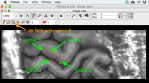
Dependent on the number of slices and the size of the region of interest, this can take 3 min up to 2 hours.

3.) Calculation of cortical depths

Relative cortical depths can be calculated in LAYNII. Below is the description on how to use LN_GROW_LAYERS.

a.) Download the all the files with from github E.g. with the command:

 git clone https://github.com/layerfMRI/laynii

b.) Compile it in the LAYNII folder with:

make LN_GROW_LAYERS

c.) Execute it with:

./LN_GROW_LAYERS -rim rim.nii

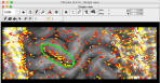
The result should look like this.

The number of 20 cortical depths in kind of arbitrary. It is a compromise between minimizing the above described partial voluming effects and keeping the datasets at manageable file sizes.

Note on single slice data (e.g. for Shinho Cho ): when the “-threeD” flag is not set, the program LN_GROW_LAYERS estimates the layers on a slice-by-slice basis. This is done assuming that the slice direction is the third dimension in the nii header according to the default of x-y-z,as phase-read-slice. If your data are not stored like this, consider using the “-threeD” option in LN_GROW_LAYERS. Alternatively, the dimentsion can be exchanged with fslswapdim input x z y  output.

 4.) Extracting functional data based on calculated cortical depths

The activity values across the different layers can now be extracts by pooling voxel values within every singe one of the 20 ROIs.

This can be done in AFNI with the following command:

#get mean value
3dROIstats -mask equi_dist_layers.nii -1DRformat -quiet -nzmean $1 > layer_t.dat
#get standard deviation
3dROIstats -mask equi_dist_layers.nii -1DRformat -quiet -sigma $1 >> layer_t.dat
#get number of voxels in each layer
3dROIstats -mask equi_dist_layers.nii -1DRformat -quiet -nzvoxels $1 >> layer_t.dat
#format file to be in columns, so gnuplot can read it.
WRD=$(head -n 1 layer_t.dat|wc -w); for((i=2;i layer.dat

The result is a text file with three rows. The Mean signal across layers and the standard deviation across all voxels in that layer.

Now you can plot the content of the simple ASCII file. E.g. with this gnuplot script. 

 

Comment on LAYNII versions

This blog post is written and tested for LAYNII versions v1.0.0- v1.5.6.