SS-SI VASO pitfalls in visual cortex

With respect to high-resolution VASO application, visual cortex is very unique. I found it to be a challenging area. However, because of its high demand, I have been working on is with multiple collaborators. The most important pitfalls of SS-SI VASO in visual cortex that I came across in these collaborations are discussed below.

The take home message tat I learned from manny experiments is:

1. Use axial slices with the phase encoding direction A>>P.
2. Watch out for negative voxels.
3. Invest a lot of effort in optimizing GRAPPA parameters, its worth it.

Anatomical challenges

Visual cortex is one of the thinnest cortical areas there are. Its about 1.8-2 mm thick and it is highly convoluted. Hence it is not straight forward to separate superficial and deeper layers. Small isotropic voxels are needed.

In collaboration with Jozien Goense in 2012, I investigated the necessary resolution to isolate upper and deeper layers in V1. Only at about 0.5 mm voxels, I started to see the deeper layer IV. for comparison, in M1, layers can be visually separated at about 0.5 mm resolutions and higher.

The higher spatial specificity of VASO compared to BOLD start of become visible at about 0.8-0.9 mm resolutions.

Because V1 is so heavily convoluted, isotropic voxels must be used.

Physiological challenges

The visual cortex has the longest arterial arrival times compared to any other cortical area. Hence the inflow-effects (see also section of inflow effects here) are relatively easy to avoid.

However, in some participants, we still saw some isolated occurrences of inflow effects. Since inflowing blood magnetization is in equilibrium, the contaminated voxels are very bright. In my personal experience this could happen when participants have an unfortunate head position. It helps when they have their chin on their chest.

This slideshow requires JavaScript.

These inflow effects of large arterial vessels are usually not very challenging in fMRI. 1.) They can be easily identified based on raw EPI signal intenities and removed. 2.) These voxels are refilled with fresh blood with activation and rest conditions. So, they do not contaminate the functional contrast.

To be on the safe side, I would advise a inversion-pulse phase skip of 30% and a inversion pulse amplitude above 90% (if SAR allows).

Negative Voxels

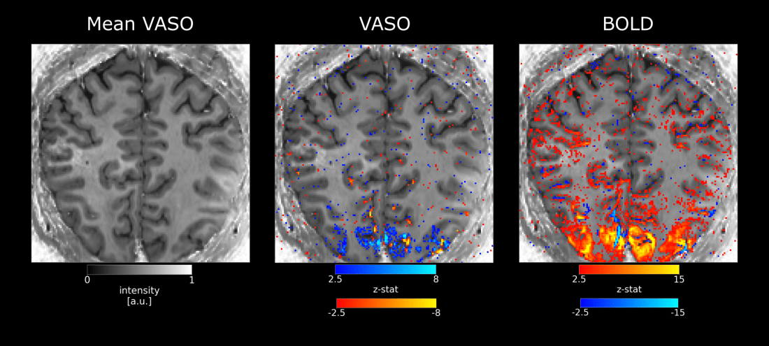
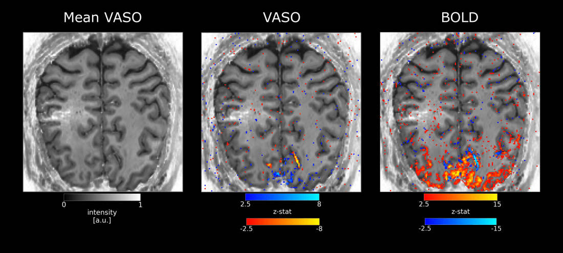
In the visual cortex (more than in other areas) it seems that there are sometimes voxels with contradictory signal changes. E.g. it voxels that overlap with bright baseline signal (indicative of arterial inflow). CBV changes seem to be negative. This strange behavior however does not solely seem to be explainable by inflow effect, as BOLD also shows negative (or reduced) signal changes. Below examples are kindly provided by Sebastian Dresbach.

Time courses

I found the hemodynamic response function and the time courses in visual cortex harder to interpret than in other brain areas. For may, tasks the time course do not simply consist of a ON-period and OFF-period but instead there are strong sensitivities to the transition periods. This results in apparent oscillations that have a similar magnitude as the overall activity change.

These apparent oscillations can confuse the GLM (whether or not the time derivative is included as a regressor or not). In some instances, I found that the strong transients upon stimulus cessation can actually result in a negative beta value.

I found a combination of three strategies helpful to minimize the effect of these oscillations on resulting activity profiles.

1. Use long trial durations. 50-60 sec trial durations (activation and rest) are the bare minimum. Only for longer trial durations the oscillations are averaged out.
2. Do not use the temporal derivative of the design matrix as an additional regressor in the GLM.
3. Collect the respiratory signal to rule out task-related breathing patterns.

Readout challenges

The visual areas are are located as an unfortunate location for most readout orientations. For axial slices, they are at the periphery of the FOV.

Due to limitations of peripheral nerve stimulation of large body gradients, a phase encoding direction in left-right direction comes a long with slower allowed readouts.

Additionally, for the channel alignment of the 32ch nova coil, GRAPPA acceleration is more efficient in anterior-posterior direction than left-right.

Thus the tSNR is higher for axial-like slices, despite the fact the matrix size is bigger that way.

GRAPPA challenges

• Since the visual areas are in the periphery of the FOV in axial slices, I found it advantageous to use lager GRAPPA KERNELS. E.g. a kernel of 5×6.
• Since the large axial slices is harder to shim, a single delay of odd and even k-space lines cannot properly capture the EPI Nyquist ghosting. Thus I found it helpful to use a “local” phase correction.
• For GRAPPA 3 in EPI with echo-spacings that are close to the acoustic resonances, I found it very beneficial to use very large regularization parameters. E.g. NoiseReduction I = 2000.
• As always, also in V1 protocols, I find FLASH GRAPPA slightly better than FLEET GRAPPA in 3D-EPI.

Good protocols tested in 2017

We had good experiences with the following two protocols:

• Tilted axial, phase encoding direction A>>P, 0.8×0.8×1 mm resolution, PF 6/8, with 8 iterations POCS, 22 slices, TE 24ms, TR = 2296, strong fat sat, phase skip 30, FLASH GRAPPA 3 in plane.
• Tilted axial, phase encoding direction A>>P, 0.8×0.8×0.8 mm resolution, PF 6/8 with 8 iteration POCS, 22 slices, TE 24ms, TR = 2535, strong fat sat, phase skip 30, FLASH GRAPPA 3 x 2, with CAIPI 1/2.

A complete list with all used parameters is given here: https://github.com/layerfMRI/Sequence_Github/tree/master/V1_VASO_layers

These data were acquired together with Yuhui Chai.

Good protocols tested in 2018

In collaboration with Insub Kim, I evaluated an even further advanced set of new protocols in July and Aug 2018. They are designed to have enough coverage to contain three ROIs: V1, V5 and LGN:

The results of a sequence comparison are depicted below.

The complete protocol-pdfs of those sequences can be downloaded here.

Example Data:

Example of both sequences can be downloaded here.

The data quality is not the best but usable:

Example data (raw and processed) are openly available on OpenNeuro 10.18112/openneuro.ds001547.v1.1.0.

Availability of the sequence.

For high-resolution applications, I would highly recommend to use the VASO preparation in combination with a 3D-EPI readout. For VB, this sequence is largely implemented from Ben Poser and the binaries can be shared with everyone via C2P. The sequence is developed for VB17. For VE, there is a sequence with a 3D-EPI readout from Ruediger Stirnberg in Bonn (see https://layerfmri.com/2021/02/22/vaso_ve/). If you are interested in the binaries of any of those sequences, contact me via layerfMRI@gmail.com.

Gentle reminder

The tSNR of VASO it 50%-60% of that of BOLD. with a smaller signal change of VASO compared to BOLD this leaves the VASO CNR in the range of 30% compared to that of BOLD.

Acknowledgments:

This work is done in collaboration with multiple people. I want to thank them for their input. Even though no successful submillimeter study with VASO in V1 been exceeded the piloting phase and no abstract has been accepted until now, a lot of work has been invested (listed in chronological order).

• Robert Trampel. Is the person who stated to look at layer-fMRI VASO in V1 with me since years. Looking back I found first attempt to to VASO layer fMRI in V1 in my monthly work report of July 2012: 1 mm resolution with 2D-EPI.  Ever since, we have been trying to get VASO working robustly regularly every few months.

• Eli Merriam and Zvi Roth is collaborating on this since June 2017. They are interested in VASO in order to measure the biological point spread function with rotating rings in V1. They have been scanning 10-20 participants in the last year. They see significant task-induced signal change. However, they are limited by (1) low tSNR of VASO, (2) time-shifted responses of VASO compared to BOLD, and (3) voxels that show the negative signal change.
  

  

• Yuhui Chai is collaborating on visual layer VASO since January 2018 using VASO regarding flickering frequencies across cortical depth in visual cortex. Yuhui did a comparison study of VASO and GE-BOLD in 3-6 participants. He sees that the VASO layer profiles look very similar compared to BOLD. They only differ in the most superficial layers.
• Markus Barth and Atena Akbari are using the same sequence with slightly different acquisition parameters at the 7T in Queensland and have an OHBM abstract about it.

  

• Daniel Haenelt and Robert Trampel and received our visual VASO protocols to use it for V2-stripes in Leipzig.

  

• Marcello Venzi and Kevin Murphy are using high-resolution VASO to investigate the neuro-vascular coupling in the visual system during visual task and during hypercapnia breathing challenges. 

  

• Won Mok Shim and Insub Kim visited NIH in July 2018 to set up a high resolution VASO protocol to investigate MVPA with orientation preference. They find that orientation decoding was possible with similar accuracy in VASO and BOLD.

  

  corresponding ROI:

  

• Saskia Bollmann and Jonathan Polimeni are also using the same sequence to pinpoint the underlying contrast mechanism of VASO with first successful experiments.