VASO FAQ

Authors: Renzo Huber and Rüdiger Strinberg.

Background

This page describes the use of a VASO sequence for SIEMENS scanners with the software platform VE. This sequence uses a 3D-EPI readout and is written by Rüdiger (Rüdi) Stirnberg and Tony Stöcker (DZNE, Bonn).

0.) I have a question about the sequence, how can I get an answer?

We are truly excited that the 3D-EPI VASO sequence has been shared already with a few dozen research labs already. We apologise that sometimes, due to the sheer amount of questions, there is a considerable time lag of answering VASO-related questions via email. Thus, if you have a specific question, please consider the following possible ways to obtain an answer.

• Please check the list of frequently asked questions below.
• Many questions about various sequence parameters can be addressed by simulating the sequence with the binaries that you have in you own virtual environment. See question 14.) for instructions on the simulation in poet.
• You can always ask questions in the comment/discussion section below, which might then be answerable by other users.
• There is a regular VASO walk-in hour via Zoom on Thursdays at 4pm UTC (winter time). Please register (renzohuber@gmail.com). Accompanying data can be uploaded here.

1.) Where can I find already tested protocols? 

Tested protocols for 3T Prismas and 7T Terras are collected on Github for standard layer-fMRI acquisitions (visual, motor, whole brain) here: https://github.com/layerfMRI/Sequence_Github/tree/master/VE_3DEPI and here: https://github.com/layerfMRI/Sequence_Github/tree/master/Terra_protocolls.

Note that these protocols are optimized for high resolution fMRI and thus, these protocols are at the limit of what the gradient performance and resonances allow. If you want to set up your own protocol, check out the tips given in question 22 (below).

2.) Can I do VASO imaging in the auditory cortex?

While the arterial arrival time from the feeding arteries to the microvascular vessels in the parenchyma is long enough to apply VASO in the auditory cortex, the pulsation of the transit vessels introduce physiological noise in the 3D-EPI readout. Thus, we found it very challenging to do layer-fMRI with 3D-EPI VASO in the auditory cortex. But it is possible within limits. We found sagittal protocols with phase encoding direction (A<<P) most efficient. See examples here or here.

3.) Can I do VASO imaging in the hippocampus?

No, probably not. The hippocampus is not only very challenging for conventional high-resolutions EPI (see example here). But it is particularly challenging for layer-dependent VASO. To my knowledge, there is only one study succeeding with VASO in the hippocampus. This study uses 3T scanners with body transmit coils and low resolutions and still needed to acquire multiple TIs to account for inflow effects.

As of 2023 there are at least four groups that are aiming for layer-fMRI VASO in the hippocampus. One of them was kind enough to share their protocol and scanner screenshots. Protocol pdf and png are included in the Github repository.

4.) Can I do VASO imaging in the amygdala or LGN?

No, the arterial arrival times of the amygdala and LGN are way too short to make VASO work without serious sequence development investment (e.g. pTx, separate labeling coils, and/or novel VASO approaches).

5.) I want to use the VASO sequence to guide gray matter segmentation. Which sequence parameter should I use to obtain the best structural contrast?

While the functional VASO data often have a nice T₁-weighted contrast, this feature has not been within the focus of the current VASO implementations. The functional VASO protocols are solely optimized for the best blood volume contrast, and the descriptions by Ruedierg Stirnberg [2020] are in turn optimized for the functional contrast. So far, we have not developed specific protocols that are optimising both at the same time. Thus, we do not have specific recommendations.

Generally speaking, in IR-EPI, the excitation flip angle that provides the best GM-blood contrast in VASO is generally higher than the flip angle that provides the best GM-WM contrast.

Thus, a good starting point to optimise the structural contrast of VASO protocols, is to reduce the flip angle. Setting the flip angle scheme (special task card) to 0, will results in an amplified GM-WM contrast. If you have a good protocol, we would very much like to include it in the open protocol collection.

6.) Which TI1 and TI2 should I use?

Overall, it doesn’t really matter too much for the quantitative VASO signal change and the local specificity of the contrast which exact values are used. As long as TI1 is smaller than the blood T₁ and as long as TI2 is larger than TI1, there should be a significant VASO signal. 

While VASO was originally proposed as a blood-nulling method (Lu et al. 2003), over the last 15 years is has been generalized to a more general T₁-contrast without specific blood-nulling requirements. Early VASO versions without blood nulling used a T₁-selective GM-nulling procedure to estimate an inverse VASO contrast (Shen et al. 2009; Wu et al. 2008). Later on, the VASO formalism was further generalized to extract CBV changes at any inversion time (Ciris et al. 2014). This literature has shown that the experimental trick of blood-nulling is not the only way of obtaining a CBV-weighting. In fact, as long as there is a different T₁-weighting between the extracellular signal and intravascular signal, any volume redistribution between these pools of z-magnetization, will result in a VASO signal change.

In everyday practice, most VASO users found it helpful to keep the TI1 above 650ms (later than the GM nulling for most TRs at 7T).  At 3T, the TI can be even a bit shorter. 

In the sequence’s protocol editor, the ultimately used TI1 and TI2 values are derived based on the “inversion-delay” in the special task card and can be viewed as read-only parameters in the contrast task card. Note that some pilot protocol pdfs (version < Maastricht4) did not depict the parameter of “inversion delay” in the contrast task card. 

Almost all of the tested protocols so far use inversion delays between 500 ms and 900 ms.

7.) The sequence is installed and starts OK, however after the first images, the scanner stops with the error message ”Preparation of Image Reconstruction System Failed”. Even for the default protocol,

As of July 27th 2020, this issue is solved with a new VASO MOSAIC functor. For previous sequence versions, see the text below.

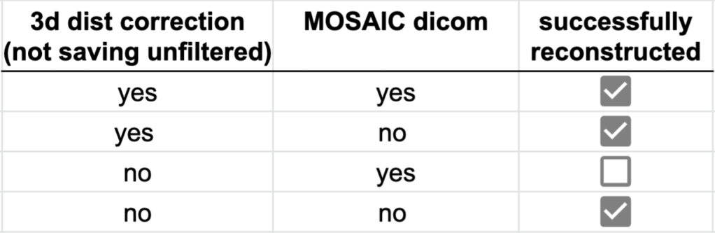
There are multiple possible causes of this problem. It would be best to make sure that all the reconstruction files are stored at the right location and that the sequence parameters are exactly like in one of the tested protocols (ALL parameters). Usual suspects are:

1. external PC, per series.
2. use: Modify IcePAT
3. Try to use Distortion corr. with 3D and not saving unfiltered images.

The following combination of image reconstruction parameters have been tested:

One work around that is a it cumbersome by has always worked for me is to runs the sequence without reconstruction and then. Reconstruct the data retrospectively:

• ideacmdtool -> Empty ICE program (6)-> OFF

• run experiment
• ideacmdtool -> Empty ICE program (6)-> ON
• twix -> retrorecon

If this is all set right and still does not work, it would be helpful to know, if it also fails with a number of TI = 1 (indicative that there is something wrong with the loop-counter for the TIs). If so it would be helpful to get the error message in the log viewer e.g. with something like “file not found”?

The respective retro-recon parameter that allows you to change the distortion correction mode is called sDistortionCorrFilter:

• 1 = no distortion correction filter
• 2 = 2D distortion correction
• 3 = is set to 4
• 4 = 3D distortion correction

The distortion correction is applied based on the file C:\Medcom\MriSiteData\GradientCoil\coeff.grad

8.) Which software baselines do you provide sequences for?

Until now, we have compiled the VASO sequence for:

• VB17b (Maastricht 3 version)
• VE11C and VE11E (Prisma)
• VE11K (some of the first first installed Terra scanners, all upgraded by now)
• VE12U (current standard Terra, before the 2021 upgrade to SP01)
• VE12U_AP01_F50 (7T plus, Terra after upgrade from VB)
• VE12U_SP01 (aka, N4_VE12U_LATEST_20181126_P13)
• VE12U_AP02 (Feinbergatron, currently only for sub version: Feature 22)
• VE12U_AP03 (10.5T), not yet.

Since the sequence is written in Bonn very independently from SIEMENS, it is not too hard to compile it for Syngo versions that are not listed yet. However, since the setup of a new virtual box including MARS can get quite involved, we would prefer access to an iso installation file to compile it for you.

9.) Most of the tested layer-fMRI protocols have a limited FOV. What is the best approach for alignment with whole brain structural data?

For the lack of better options, we mostly segment the GM voxels manually in the T₁-weighted contrast of VASO. This is often guided by auxiliary structural data that are area fashion registered to each other. On this blog post, it is explained how we register small FOV VASO data to whole brain data.

11.) I still use a VB 17 scanner. How can I optimize my VB 17 sequence?

This FAQ site refers to the DZNE sequence that has almost exclusively distributed for VE scanners (e.g. Terra 7T and Prisma 3T). If you are using a VB17 scanner (e.g. classic MAGENTOM 7T, Trio), you are probably using a completely different sequence baseline that has been distributed via Benedikt Poser. The usage of this VB sequence is explained on a different blog post here.

While the DZNE sequence is mainly supported for VE, some experimental versions of it can be compiled for VB 17 too. Those VASO versions are not fully vetted (yet) and used for exploratory purposes only.

10.) I am running an older VASO version of the sequence. Can we set up a new C²P to also get access to the updated version?

It is usually not necessary to make a new C²P (core-competence-partnership, CCP, C2P) to receive updated sequence, even when they have new functionalities (e.g. MAGEC). Reach out to Rüdiger Stirnberg (Ruediger.Stirnberg@dzne.de) and/or Renzo Huber (renzohuber@gmail.com) about the request for an updated sequence.

12.) What does the flip angle scheme mean?

In the VE sequence, the variable flip angle scheme is implemented by means of an extra field in the special card: varflip scheme. The special card parameter that determines the flip angle scheme is called: VarFA/MAGEC (in older versions this is called varflip).

• 0 means that there is a constant flip angle across segments. The FA in the contrast task card refers to the constant FA in degrees.
• 4 means that there is an increasing FA scheme. This is done to increase SNR, while minimizing T1-related blurring as explained here. The number of FA in the contrast task card then, refers to the largest (last) FA in degrees.

Since the variable flip angle is adjusted for one T₁ compartment only, other T₁ compartments (E.g. WM and GW) will have a different point spread function. Often, this can result in an edge enhancement artifact, as shown below.

This effect can be partly accounted for by applying a corresponding weighting in k-space of retrospectively, with the “-laurencian’ option in the LAYNII program LN_DIRECT_SMOOTH.

13.) Could not load sequence on scanner (green files)

It can happen that you put all the sequence and reconstruction files in the right places at the scanner. And for some reason they seem green. And then, when you run the sequence, you get the error message “could not load sequence” with a few follow up errors.

This is an unfortunate result of Windows trying to be more safe. It has to do with the fact that Ruedi and Renzo usually send sequences via compressed zip files from OS X to be uncompressed on Windows file systems. Namely, it can happen that Windows does something semi-stupid and re-encrypts the files for you on your windows system, and thus they appear green in Windows Explorer.  The solution of this is the following simple steps (in update mode): 

• Right-click the green folder, and choose Properties
• Click the Advanced button
• In the Advanced Attributes window that pops up, UNcheck the “Encrypt contents to secure data” checkbox.
• Click OK, and when it asks if you’d like to apply this change to all files in the folder, say yes.

Dependent on the state of the MRIR after the above errors, you might need to restart the image reconstruction.

14.) I only have the binaries of the sequence, how can I simulate what the scanner does? E.g. to check for acoustic resonances?

You can simulate the sequence with the binaries in your virtual box by following the steps below.

1. Transfer the binaries by setting up a shared folder between VM and host OS.
2. Copy sequence dll (i.e. rslh_ep3d_vaso.dll) into Z:\n4\x86\prod\bin
3. From the IDEA VM, start VE12U IDEA (IDEA.Net) 
4. From the start menu select CS0/CS1/CS2 (whichever you use) for VE12U. 
5. At the prompt type ‘sys’ to set system type to Terra-XR.
6. Start the protocol editor by typing ‘poetr /online \n4\x86\prod\bin\rslh_ep3d_vaso.dll’
7. Now you can edit and save or open protocols.
8. Start a simulation by going to Tools>SIM…

15.) Is it possible to use this sequence with just one inversion time, and thus achieve VASO fMRI with a shorter TR?

No! Unfortunately, at 7T any EPI readout will always have an effective finite T2*-weighting that introduces BOLD contaminations, counteracting the VASO signal. For TEs of 20ms and larger the overall BOLD signal magnitude is already as big as the VASO signal decrease, completely canceling any functional signal change. For shorter TEs, down to TEs of 7m, the BOLD signal dominates in larger draining veins, while the VASO dominates in the parenchyma. Even for EPI with zero echo times (e.g. Spirals) we found that the unwanted T₂^* weighing of the outer k-space data can introduce serious BOLD weighting. Thus, a proper BOLD correction with interleaved acquisition of BOLD and VASO is always advised. Only for very low field strengths of 1.5T, (where VASO was originally discovered) such BOLD correction methods are not necessary.

16.) I cannot find all the parameters in the special card that are given in the protocol.

Many of the special card parameters are only visible, when other parameters are set. E.g. the “Saturation RF” field only becomes visible when a fat-sat pulse is selected in the contrast task card or a regional saturation pulse was added. And some partial Fourier parameters are only visible when Partial Fourier is used etc. The varflip scheme is only visible when an IR mode is selected in the contrast task card (for versions > RenLay8) etc. Note also that the sequence has gone through a few changes in nomenclature over the last year. If you are not using the latest version and want to get access to it, reach out to Rüdiger Stirnberg (Ruediger.Stirnberg@dzne.de) and/or Renzo Huber (renzohuber@gmail.com)

17.) Depending on how I export the dicoms and convert them to 4d nii time series, the ordering of VASO and BOLD is not right. What can I do to fix this?

As of July 2022, this issue is solved by means of a new MOSAIC decorator. In case you are using a sequence version that is older than this, the below text might be helpful.

The sequence acquires the images concomitantly. Thus, each pair of BOLD and VASO is in the right order, however, it can happen (mostly for the sequence version of maastricht 4 and later) that a BOLD is written to memory before the VASO or vice versa for each pair. E.g, while the correct order of the volumes should be: V₁, B₁, V₂, B₂, V₃, B₃, V₄, B₄, V₅, B₅….. it wrongly is written as V₁, B₁, V₂, B₂, B₃, V₃, B₄, V₄, B₅, V₅. This can be avoided, if the dicom to nii conversion is specifically done on VASO only and on BOLD only, separately. The dicom header that indicated whether a volume is BOLD or VASO is: DICOM -> CSAImageHeaderInfo -> ICE_Dims. “1_1_1_1_” stands for VASO and “1_1_1_2_” stands for BOLD. This conversion script writes each time series into separate nii files in the right order based on this dicom header: https://github.com/layerfMRI/repository/blob/master/conv/conv_Kronbichler.sh

Addendum: Mac users with version of BigSur (11.6) alt newer report issues with isisconv. One alternative AFNI conversion option is as follows (thanks to Andrew Persichetti for this solution).

Dimon -quiet -sort_by_acq_time -infile_pattern "mr_0016/*.dcm" -dicom_org -gert_create_dataset -gert_to3d_prefix testMosaic.nii

ADDENDUM: This issue is fixed as of June 2022

As part of the OHBM Hackathon 2022, an updated VASO MOSAIC functor was developed that sorts images with VASO and BOLD contrast in separate time series. (blog post about Hackathon). If you want to use this functor too, just reach out to Rüdiger or Renzo to receive the binaries.

For the installation, you need to follow the steps at the scanner:

1. Enable the embedded controlGUI
2. execute ideacmdtool 2 (this is the PAS unload)
3. execute ideacmdtool 2 (again)
4. Replace IceMosaic2D3D.dll and libIceMosaic2D3D.so in C:\MedCom\MriCustomer\ice\
5. Execute C:\MedCom\bin\rti.exe terminateComp Cocos (this safes you the full reboot)
6. Execute C:\MedCom\bin\rti.exe runComp Cocos

18.) How can I adjust the inversion efficiency to minimize inflow of fresh blood?

Early VASO papers regularly mention the necessity to minimize inflow of fresh blood by means of adjustable inversion efficiencies and so called phase skips (https://layerfmri.com/tr-foci-pulse-optimisations/). While this was vital for the very early (24ch) Nova RF coils, with which the SS-SI-VASO was originally developed, this has no longer been a limiting factor for high resolution VASO with the new generation of Nova coils. Thus, the latest VASO sequence versions no longer have the option to adjust the inversion efficiency by means of a phase skip. This, means that the latest VASO versions always use a full inversion. This maximizes the GM CNR for VASO. The residual inflow effects are solely occurring in transient pial vessels (see here: https://layerfmri.com/negative-voxels-in-vaso/) and can be easily avoided by means of a GM mask.

The unavoidable inflow effects in the deep brain structures are way too strong and way t0o fast that the adjustable inversion efficiency could account for it.

19.) Is it possible to use this sequence with two inversion times to estimate the baseline CBV?

No! Unfortunately not. The SS-SI VASO sequence can only be used to estimate quantitative changes of CBV.

At high magnetic field strengths, the variance of T₁ between different layers of GM and the variance of T1 between different brain areas are comparable as the variance of T₁ values of blood and GM. Thus, a simple multi compartment model of blood and extravascular tissue is underdetermined. Higher-level models with more inversion times, however, are being developed for exploratory purposes. 

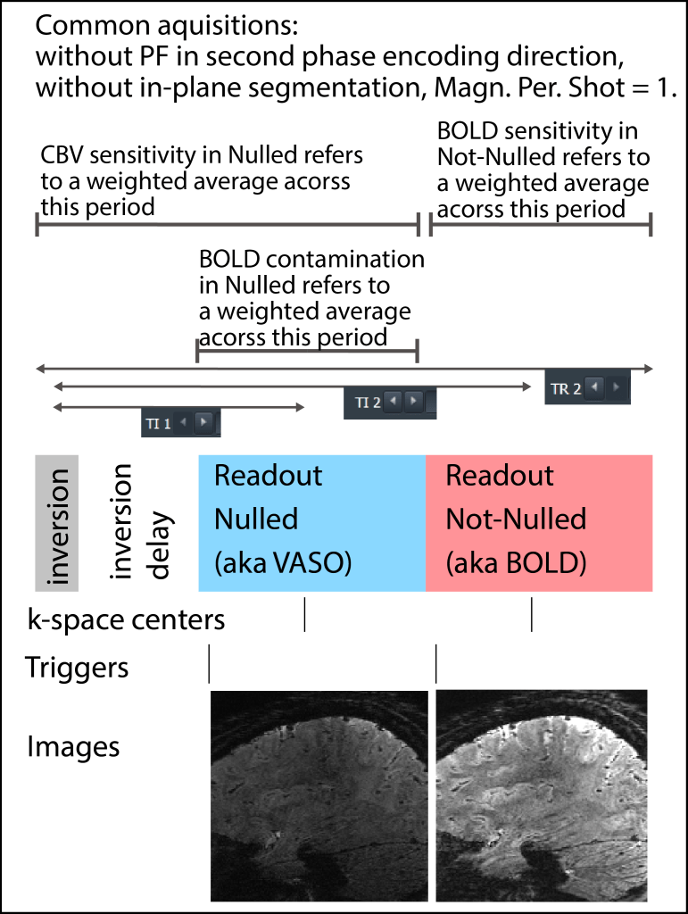
20.) The protocol gives me two TRs (TR1 and TR2), do these refer to the TRs of BOLD and VASO respectively? Which TR should I use to synchronize the logged triggers with the task? What is the TR looping structure?

The TR1 refers to the time between two consecutive 3D-EPI excitation pulses and is thus usually very short (<100ms). This is comparable to common 3D-EPI BOLD sequences. 

The TR2 refers to the time of acquiring all complete volumes of an entire inversion recovery cycle. This is comparable to volume acquisition time of an MP2RAGE sequence. The TR2 refers to the effective temporal resolution of each pair of Nulled/Not-Nulled images. Thus, this is the double of the time of the TR-naming convention in comparable ASL sequences. The TR2 is double the time that would be the TR in the COBIDAS and BIDS nomenclature.  If you extract the Nulled and Not-Nulled time courses as a combined nii 4D-file, the header TR of this nii should be set to be half the TR2.

Note that the VB17 VASO version that was shared via Benedikt Poser uses a ASL-type TR nomenclature.

The triggers are played out at the beginning of each volume acquisition, each inversion image per TR. Thus, if in-plane segmentation is used, pairs of triggers are interspaces with relatively long dead times. 

Example TR loops with and without in-plane segmentations (zoom in):

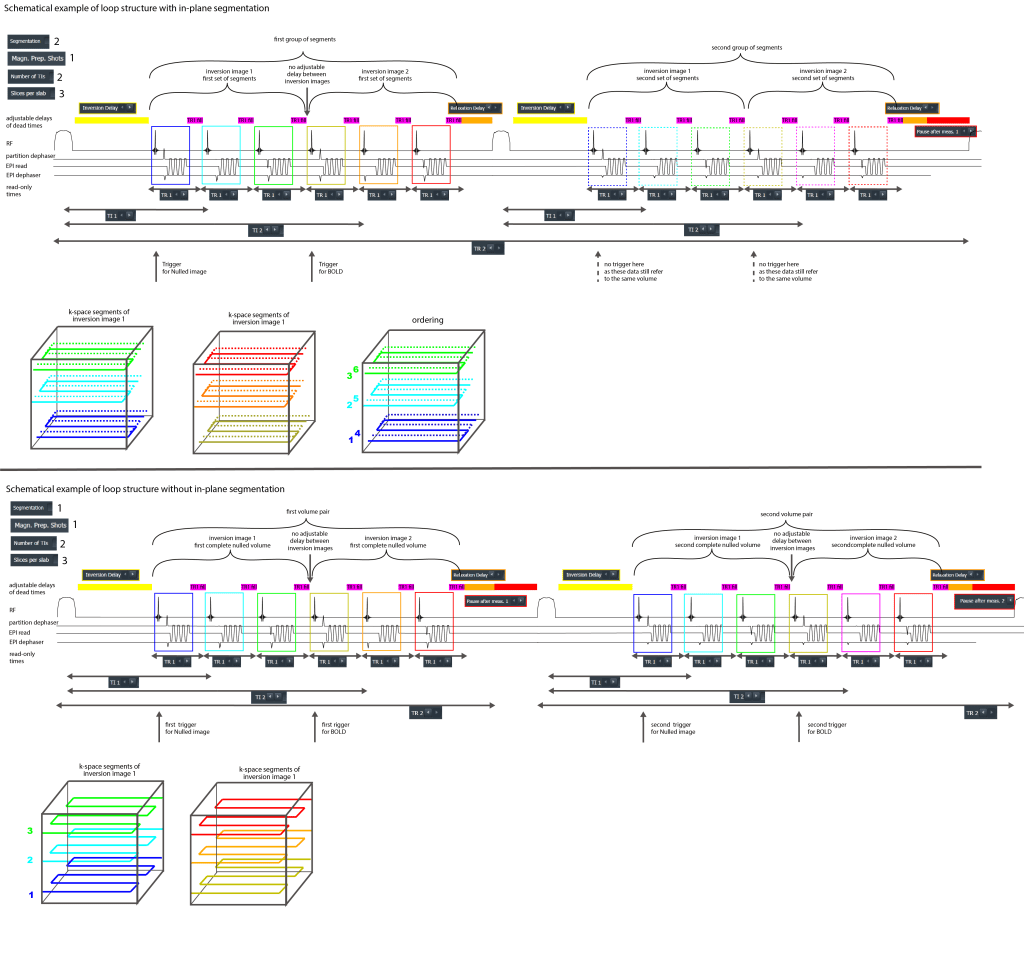
If you are following the VASO analysis from Renzo (outlined here) that uses separate nii 4D files of Nulled and Not-nulled data with temporal upsampling by a factor of 2, the nii header TR should be half of TR2 from the scan protocol.

22.) What do I need to consider when I want to set up my own protocol?

While it is recommended that you use previously tested acquisition protocols available on Github, those protocols might not always fit your needs. The protocol templates mentioned in question 1 (above) can act like a solid starting point for other cortical areas too. If you want to setup your own protocol from scratch, it is advised to go through the steps outlined below:

• Start adjusting parameters with long TR, long TE, low bandwidth, few slices.

Fat saturation

• If the slab-thickness allows, start with water excitation instead of fat saturation (the latter reduces 3D-EPI tSNR considerably [Stirnberg2016] by MT):
  • For protocols with whole-head coverage, you could try: sagittal slice orientation, RF pulse non-selective, single hard pulse water excitation (Special card > water exc. > singe RECT) [Stirnberg2016].
  • For slab protocols (thin or larger whole-brain), use either Binomial 1-2-1 (Contrast card > water excitation), or Binomial 1-1 (Special card > water exc. > Bino-11) [Stirnberg2017].
  • “Long single RECT” and “Long Bino-11” lead to more inhomogeneous excitation, but can be helpful to reduce peak B1/ obtain an acceptable RF BWT product at high-fields.

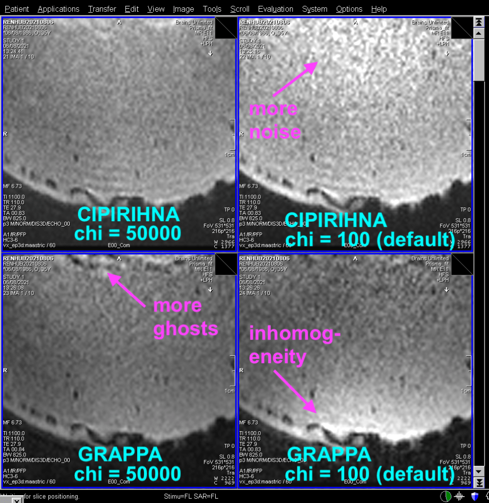
Acceleration and CAIPI

• PAT mode CAIPIRINHA (activates improved IcePAT reconstruction, even if CAIPI shift = 0). This means that the GRAPPA unaliasing is done in 3D, in contrast to two consecutive 2D unaliasings as done in PAT² (referred to as GRAPPA).
• Tooltip over Boolean parameter group on special card gives various infos, e.g. about the EPI trajectory. Skipped-CAIPI notation [Stirnberg2020].: S.R1xR2zD (S=Segmentation factor, R1=undersamplig factor along PE, R2=undesampling factor along slice, D=CAIPI shift along slice). For convenient plotting of the sampling patterns for your combination of acceleration, segmentation, and CAIPI shifts, Check out Skipped-CAIPI visualization on github.

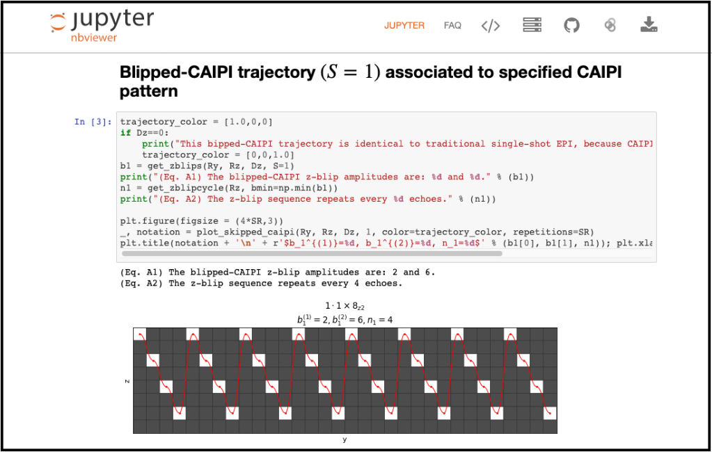
• The optimal CAIPI pattern depends on slice orientation and receive coil used. Rule of thumb: rather accelerate by R2 (min. TR, analog to multiband factor in SMS-EPI). Use R1>1 only if needed to achieve short TE despite large matrix size (layer-fMRI), for instance. Even in this case, it can be useful to rather employ a segmentation factor > 1 together with a small R1 to accomplish small EPI factors/large PE-blips with a better suited undersampling pattern [Stirnberg2020]. This is particularly true for VASO.
• Reference scan mode (has an effect on noise increase and residual parallel imaging artifacts). Rule of thumb:
  • if final image has EPI-typical geometric distortions (e.g. 1.1x6z2, y-blip=1, relatively large EPI factor), select EPI/Separate (realized by segmented dual-polarity ACS [Stirnberg2020])
  • if final image has little distortions (e.g. 2.2x3z1, y-blip=4, relatively small EPI factor), select
  • GRE/Separate (realized by FLASH readout). This is recommended for low bandwidths with layer-fMRI.
  • Don’t forget to adapt the PATRef flip angle, e.g. according to Ernst T1 tooltip on Special card Follow PATRef prep. shots recommendation given in by Ernst T1 tooltip. Max. is fine, even if recommendation is higher, and not too long.
  • Note that the Ernst T1 is ‘only’ a tooltip. It calculated the Ernst angle for you. However, if you want to follow the recommendation by the tool tip, you still need to set the FAs accortingly in If you want to follow the Ernst angle recommendation in the tooltip, you still need to adjust the value accordingly (e.g. PATRef FA).
• If series is very large, consider activating “Matrix optimization: Performance” on System Card/ Miscellaneous (very long scans may abort otherwise). in this case prescan normalize should not be activated.
• Be conservative with partial Fourier. If used to realize shorter TEs, keep “Min. TE if PF” enabled. Too liberal partial Fourier might result in in unwanted signal blurring (see this blog post).

Final adjustments

• Finally, increase bandwidth to almost max., set desired echo time(s) and minimize TR.
  • The multi-echo spacing defaults to minimum achievable, gradient-rephased TE spacing. It can be changed, once contrasts (Sequence > Part 1) is > 1. Then, the resulting multi-TEs are displayed, but can only be modified by adapting the multi-echo spacing. Note:
  • Multi-echo spacing refers to the “true” gradient rephased spacing between multi-echo EPI readouts By selecting Multi-echo shots > 1 (Routine card), a fraction of this spacing can be realized by “TE segmentation” (even without rephased multi-echoes) [Stirnberg2018].
• In conjunction with magn. prep., ext. phase correction “per series” should be used. This also minimizes (first) TE. Other options are available but not tested with magn. prep.
  • Ext. PC “per series” or “per volume” means a dedicated small 5 deg flip angle pulse and PC acquisition at the beginning of the entire series or each volume acquisition, respectively [Stirnberg2020].

23.) I changed one protocol parameter and now I cannot change it back to the value it was before.

Please be aware that this is a custom sequence and no official works-in-progress sequence. This means, some of the features are experimental. Thus, solve handlers are not implemented for every situation, which means that one may get locked up in parameter space when setting up a new protocol. By importing the sequence from scratch and following the list given in Q22, one can avoid or get out of such a “locked up” situation.

When you import the sequence from scratch, the default “minimal” protocol is designed to run “out-of-the-box” on most scanners – although far from being optimized. Depending on subject/gradient specs, however, the gradient stimulation check may give a warning or even require you to reduce the readout bandwidth (to relax the gradients).

Typically locked parameters can be unlocked as follows:

• Matrix size. If you cannot increase the matrix size to your desired choice, try varying one of the following parameters: Bandwidths/Px, phase oversampling, gradient mode. As soon as you adjusted the Matrix size you can set them back to where they were.
• GRAPPA in Ky: If the protocol editor does not allow you to switch off GRAPPA in y-direction, try increasing the acceleration factor in Kz. As soon as this is done you can lower GRAPPA factors in Ky and then lower Kz later too.

24.) The sequence doesn’t work for me. Where do I need to put the respective files?

Since version Maastricht4, there are 10 filed that need to be included on the scanner:

• MriCustomer\seq\rslh_ep3d_vaso.dll
• MriCustomer\seq\librslh_ep3d_vaso.so
• MriCustomer\ice\IceMosaic2D3D.dll
• MriCustomer\ice\IceMosaic2D3D.evp
• MriCustomer\ice\libIceMosaic2D3D.so
• MriCustomer\ice\IceDecoratorMosaic2D3D.ipr
• MriCustomer\ice\ModifyIcePatConfig.dll
• MriCustomer\ice\ModifyIcePatConfig.evp
• MriCustomer\ice\libModifyIcePatConfig.so
• MriCustomer\ice\IceDecoratorModifyIcePatConfig_ep3d_vaso.ipr

Make sure, that you placed them in the respective location while you have the Embedded Control update mode enabled. Also, make sure none of the files looks green (question 7). Never overwrite any filed that are already there, without making backups. In almost all cases, the already existing files will be fine.

25.) That is the difference of ‘non-sel. IR’ and ‘non-sel. IR HSN/T1map‘?

Note on nomenclature: non-sel. IR HSN is the same as non-sel. IR T1map. Initial VASO versions referred to it as T1map. Since version maastricht4, this is referred to as HSN.

These are two options in the Magn. preparation menu of the Contrast task card. They refer to the same IT timing and the same readout loops. The only difference is that they use different inversion pulses. The non-sel. IR refers to a sech (hyperbolic secant) pulse, which does not have the best SAR efficiency, and non-sel. IR T1map refers to a Hypersecant 6 pulse which might have a slightly lower adiabaticity close the on-resonance during the frequency sweep.

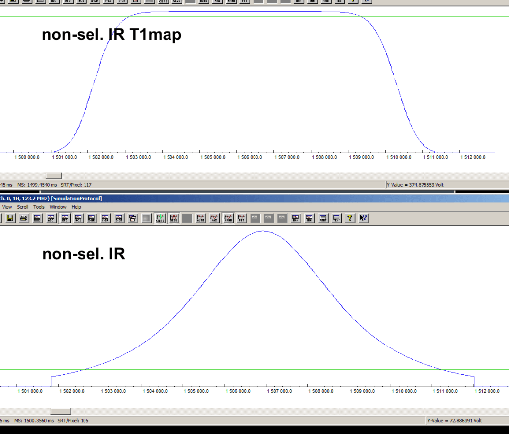
Given that VASO applications with 3D-EPI are rarely SAR limited at 7T, we would recommend the use of non-sel. IR. Collaborators have had the experience that the other options has limited inversion efficiency when the head is not deep in the RF coil (chin away from the chest to see the mirror easier).

When you are using the HSN pulse, the special card also allows you to manipulate the magnitude of the pulse. E.g. setting HSN power scale=3, results in a three fold stronger B₁⁺ magnitude.

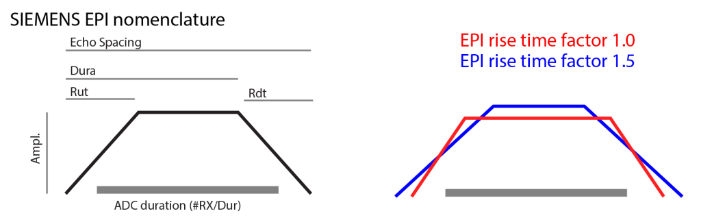
26.) What does the parameter EPI rise time fact do?

This additional parameter was added since version Maastricht4. It’s purpose is to allow a more flexible manual adjustment of the echo spacing (and corresponding TE) for a given readout bandwidth. It affects the gradient slew rate and the ramp sampling ratio. Besides the gradient mode, this is the only other parameter that allows adjustments of the slew rate.

Generally, a lower rise time factor allows a wider spectrum of bandwidths.

This parameter is very helpful to reduce peripheral nerve stimulation (PNS) limits after the timing of the sequence has been set up.

See also also the info blob in the special card.

27) What does the parameter ETL per RTEB mean?

The echo train length (ETL) per real time event block (RTEB). In the most cases, a value of 1 should be fine. This is a debugging parameter for the developers only.

28) What does the parameter Modify IcePat do?

Background: What is IcePat (selected with CAIPIRINHA) and what is Pat2 (selected with GRAPPA)?

In the resolution task card (IPAT) there are two selectable modes to do undersampling. CAIPIRINHA and GRAPPA. While the sequence does the same thing for both modes, the reconstruction is slightly different.

GRAPPA mode (also known as Pat²) is applying the GRAPPA unaliasing reconstruction algorithm in two dimensions in a consecutive way. The two dimensions are done sequentially. Fist, in-plane, then through plane. It is implemented as described by Blaimer (2D-GRAPPA-Operator for faster 3D Parallel MRI, MRM 2006).
CAIPIRINHA mode (also known as IcePat) is different; IcePat does the GRAPPA unaliasing in both directions at the same time. As described by Felix Breuer (2D CAIPIRINHA).

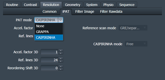
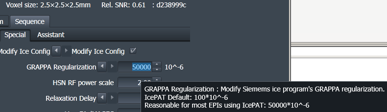
What does the special card parameter Modify IcePat do?

This parameter is only visible, when IcePat is used. I.e. When you use acceleration with IcePat (aka. CAIPIRINHA), one can modify the GRAPPA regularisation and GRAPPA Kernel size. The parameter Modify IcePat, increases the regularisation compared to the default from 0.0001 to 0.05. This is increased regularisation is considered advantageous for layer-fMRI.

Furthermore, the Modify IcePat parameter allows the user to conveniently adjust the kernel size in the file IceDecoratorModifyIcePatConfig_ep3d_vaso.ipr, if needed. Unless it is changed by the user, the default kernel size is used. Special thanks to Philipp Ehses for developing these tools.

Note, as soon a you select the check-mark of “Modify-Icepat” in the special card, we found that a retrospective reconstruction does not work without problems anymore. The only work around that I found so far to make the retro-recon work is to reconstruct it without the Modify icepat (by using the twix header from a file without using it) and instead modify the C:/MedCom/config/Ice/PATConfigurator.ini file manually.

29) The timing of TR2 does not perfectly match with the timing of the triggers.

For some protocols, and some older versions (prior maastricht4d), the TR2 timing shown in the protocol editor does not match dime difference of the triggers, that are used to synchronise the stimulation task. Usually, the trigger timing is slightly longer than the TR2 in the protocols editor (6.3-14ms longer per slice).

This problem is particularly visible with conventional fat-saturation pulses and multiple inversion times.

Without any Fat sat or with SPAIR fat-sat (fat selective inversion recovery based fat saturation) this TR underestimation does not occur.

Generally, we recommend to synchronise the functional task based on counting scanner triggers rather than absolute timing. For, sequence versions of maastricht4d and higher, the read-only field TR2 in the protocol editor should match the time periods of two triggers up to an accuracy level of 5ms.

30) Prescan Normalize, should I use it?

Many scanners (3T) have the included option of “prescan normalize” (Resolution > Filter card of protocol editor). According to the the SIEMENS’ description, the purpose of this option is to correct for B1+ bias field by means of a pair of low res 3DGRE reference scans (with the head coil and body coil receiving signals, respectively). Note however, that this filter does more than just a voxel-wise scaling of the magnitude images. This option uses is used in combination of the Roemer combination method and it produced fundamentally different (improved) phase images. And the phase images do not suffer from open-ended fringe lines.

References:

• ISMRM 2018 by Eckstein, abstract.
• Kaza et al. 2011, paper.
• PracticalfMRI blog post about prescan normalize.

Note that the option of saving both images, with and without prescan normalize are selected there are additional reconstruction limitations. For example, if “save unfiltered” images is selected for prescan normalize, the gradient non-linear distortion correction can not longer be saved unfiltered. Also, if there are more than one inversion times (e.g. in SS-SI-VASO), more than one reconstruction mode (e.g. magnitude and phase), or echo times (MEICA), the “save unfiltered” option will result in reconstruction errors.

31) What does the NORDIC parameter do?

With the increasing popularity of NORDIC-denoising for layer-fMRI VASO, we included the option to acquire reference noise scans at the end of the run. Those noise scans are necessary for NORDIC’s PCA thresholding while capturing the run-specific g-factor noise amplification. This is done by setting the excitation flip angle of the last two volumes to zero, while keeping the same GRAPPA kernel of the functional data. This noise scan can be used with the NORDIC demonising code provided by Steel Moeller (not included in the scanner reconstruction).

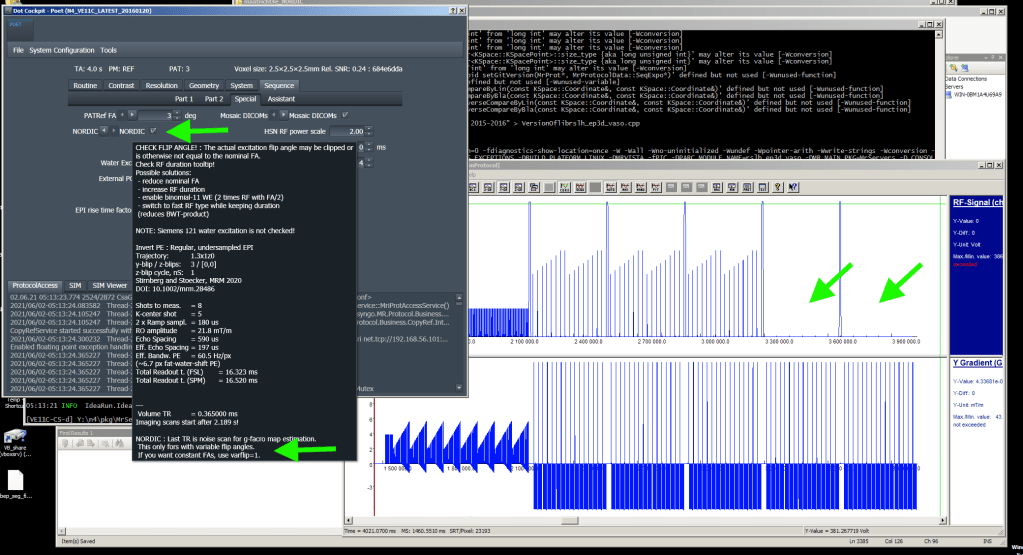
Noise scans are expected to exhibit local variation of the noise floor.

32.) How does the scanner send the triggers to stimulation environment, and how does this relate to the images after the BOLD correction has been performed?

The sequence sends triggers at the start of each readout block per volume. This means that in most cases the triggers come in pairs that are not homogeneously distributed across time.

Note that the triggers are shifted with respect to the k-space center of the respective volume.

Also note that the common equidistant interpolation in the BOLD correction analysis does not account for this shift. However, the effect can usually be considered negligible.

Also note that conventionally, the functional sensitivity of BOLD and VASO are not identically distributed across the readout block. If you select the “Sym VASO option” in the special card (accessible as of July 2022), additional dead-times are added to symmetrically spread out VASO and BOLD images.

A more detailed discussion on the BOLD of VASO can be found here and in references therein.

The image time series are written out in the order they are acquired in. This means that the blood-nulled (VASO). time series are written before the non-nulled (BOLD) time series.

33.) What does the POCS iterations parameter do?

POCS refers to projection onto convex sets and refers to a reconstruction algorithm of partial Fourier imaging (developed in 1991). This algorithm minimizes some of the resolution loss of partial Fourier imaging and is relatively robust against B0-inhomogeneities. It is an iterative algorithm that is by default only executed twice. In the presence of particularly strong B0-inhomogeneities and low bandwidths (for layer-fMRI) more iterations can be necessary. In most cases 8 iterations is a good number.

This parameter is only adjustable, when partial Fourier imaging is used in combination with GRAPPA undersampling. This parameter is not used in IcePat (aka CAIPIRINHA undersampling).

In most cases the number of iteration does not have a very large effect on the data. If any, more iterations reduce the B0-artifacts a little bit.

More information on POCS and partial Fourier imaging is provided in this post.

This parameter is kindly made available in this sequence by Phillip Ehses.

34. ) What does the GRAPPA regularization parameter do?

This is a reconstruction parameter that determines how smooth the GRAPPA kernel is assumed to be. Increasing this parameter increases the tSNR, as the cost of stronger ghosts. These ghosts are usually weaker in-vivo compared to phantoms.

More details about the GRAPPA regularization is given in this post.

This parameter is kindly made available in this sequence by Phillip Ehses.

35) Previously reporter issues

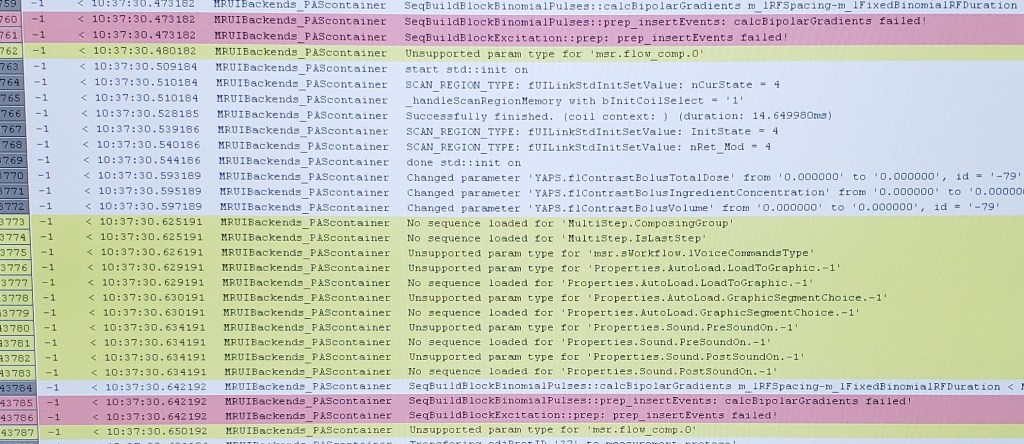
35.1) Normal error messages in the log viewer that are NOT matter of concern.

These error messages can be ignored and are provided for reference to know that they can be disregarded.

35.2) 3D distortion correction is not selected

This can be solved by selecting 3D-distortion correction. See also question 7. We are currently working on solutions to make it work without 3D distortion correction.

Sometimes (not always, though), when the distortion correction is not selected there is the following additional error too.

This error can appear with and without water excitation being selected or not.

Yet, for other occasions the same problem comes a long with an error as follows:

35.3) Sequence (or reconstruction) binaries are compiles for the wrong version.

35.4) Sequence does not run.

35.5) Protocol editor is super slow

Every click takes several seconds and the protocol editor pauses many times. This problem was specific to the VASO sequence and got resolved after the exchange of a faulty multinuclear amplifier. (Kindly provided by Cambridge).

36) What do I need to consider when running this sequence in pTx mode?

For the Nova coil: There are a few users of this sequence that already used it for layer-fMRI VASO in pTx mode. However it is important to note that there are some differences about the different Terra scanner versions and RF coil used. The Terra plus (upgraded classical MAGNETOM, Eg.g. AP01) is slightly different than the native Terra (e.g. SP01). On the Terra plus systems the ‘first level’ and ‘normal’ SAR mode are the same. So there is no way to benefit from the less conservative first level mode like on the native Terra. Thus, some AP01 users of this VASO sequence where limited by SAR in pTx and prefer the CP mode.

When you are using a custom coil, things are a bit different (Thanks to Joe Gati and Kyle Gilbert for explaining this): In fact, the 20-W/kg local SAR limit is enabled (i.e., SWD.tSupportedSARGuideline  = “IEC03,IEC02” in the coil file) in 1st level mode. However, the Nova coil does not use a local body model for local SAR calculations in pTx mode. It calculates SAR strictly on forward power, so SAR is always limited by the coil file to either the following average power limits:

• SWD.flTxAvPwrLimit_LT = 24 // [W] @ coil plug
• SWD.flTxAvPwrLimit_10s = 36 // [W] @ coil plug
• SWD.flTxAvPwrLimit_1s  = 70 // [W] @ coil plug

or to the total power times the K-factor (whichever is worse). Since the average power is not changing when you enter 1st-level mode, one doesn’t see a difference in the allowed SAR.

Also, note that when you use this sequence for small FOV slab protocols as commonly done for layer-fMRI VASO it should be considered in the B1-shim ROI. For VASO, it’s it not only advantageous to do the B1-shim over the imaging ROI, but it is also important to cover the feeding arteries. In order to minimise inflow-effects in VASO, the Hypersecant 6 inversion pulse requires about 10 mu Tesla to fulfil adiabatic and full inversion.

The feature of using a pulse-specific whole brain pTx shim for the inversion and a local ROI-specific shim for the excitation as previously applied at 9.4T VASO, is not yet implemented in the this sequence.

37) How can I adjust the pTx Shim mode?

The pTx adjustments of the VASO 3D-EPI sequence can be adjusted like the native 3D-EPI sequence or most other sequences for that matter.

For the patient-specific session-wide adjustments, you can use the System->Adjustment->Manual Adjustment settings.

For run-specific settings, you can change the settings in the protocol editor-> System-> Adjustments -> B1 Shim mode.

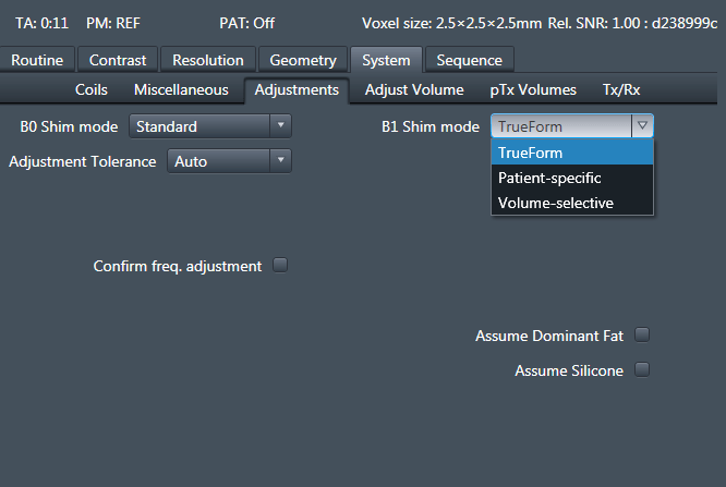
We found that for functional VASO application of the cortex the 1st level mode SAR model of TrueForm is the most advantageous setting.

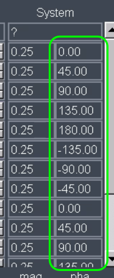
38) How can I run the sequence in CP2+ mode?

CP2+ refers to a form of CP+ mode (the + refers to transmit) that adjusts the phases of the individual channels of the circle in two rotations.

I.e. instead of the conventional phase offsets across RF channels of: 0, 45, 90, 135, 180, -135, -90, -45, etc. the phase offsets is set to 0, 90, 180, -90, 45, 135, -45, etc.

39) I cannot reproduce the shared example protocols without violating PNS (peripheral nerve stimulation) limits. What can I do about this?

This seems to be an issue with the latest upgrades of the Prisma (VE11E), which has more conservative thresholds compared to the previous version (VE11C).

Whatever you do, please make sure that the gradient mode “Performance” is selected on the Sequence/ Part 2 card. This will only let you utilize the full power of the Prisma gradients, and at the same time, the behaviour of PNS warnings and limits may change a bit compared to the typical “Fast” mode.

The strikter PNS limits on VE11E were the original reason, why Rüdier had added the “EPI rise time factor” on the special card on my 3D-EPI sequences (See question 26 above). This may give a little bit of freedom with regard to reducing PNS as that factor increases the rise time (decreases the slew rate) of the EPI readout and phase encode gradient blips. Typically a value somewhere between 1.1 and 1.2 minimizes PNS, depending on the protocol. Higher values (above 1.2) may again increase PNS, as typically the gradient amplitudes have to increase in order to account for the reduced rise time.

If playing with the EPI rise time factor won’t help after all, only reducing the readout bandwidth is ultimately going to let you reduce PNS

40) Can I use the 3D-EPI VASO sequence also for BOLD-only measurements?

While the VASO sequence of this FAQ is not really set up for BOLD-only measurements, it can be setup in away that comes somewhat close to a BOLD-only experiment. As such, if the inversion pulse magnitude is reduced to 0 and if the inversion delay is reduced to zero, the sequence will act like a BOLD-only sequence with pair of TRs. While this ‘hack’ can serve as a good first shot for a BOLD-only sequence, it is not optimized for BOLD-only and you cannot benefit from a number of optimizations and additional bells and whistles that are included in the latest DZNE BOLD sequence.

For instance:

• In the clean non-VASO, BOLD-only sequence, one can adjust the volume TR directly.
• In the clean BOLD-only DZNE sequence one will get exactly one trigger per volume.
• In the clean BOLD-only DZNE sequence one will be able to chose from more options for different phase correction modes.
• Tn a clean BOD-only DZNE sequence, there are additional half-elliptical sampling schemes that do not make sense for VASO.

Thus, if you are interested in a BOLD-only sequence, it is highly recommended that you do NOT use the VASO sequence. Rather, it is recommended that you reach out to Rüdiger Stirnberg to request a clean BOLD-only sequence.

41) Which coil combination method should I use?

We recommend to perform GRAPPA acceleration with CAIPIRINHA mode (activates IcePAT reconstruction, even if CAIPI shift = 0). As soon as this acceleration mode is selected, the reconstruction chain used int’s own adaptive combine coil combination methods. This is despite the fact that the system task card still shows sum of squares.

There are several multiple flavors of adaptive combine coil combinations possible.

1.) When pre-scan normalise is used, the adaptive combine coil combinations is done with referenced phase valued with respect to the reference RF coil. At 3T this might be the volume transmit coil, at 7T this might be the 1TX nova coil. This coil-combination method provides coil-combined phase data without open-ended fringe lines. (default when pre-scan normalize is used)

2.) Then no reference coil is available (e.g. for custom coils without TR switch or pTx coils), a simplified adaptive combine coil-combination mode is used. (default when pre-scan normalize is not used).

3.) There is a further option to use a different adaptive combine coil-combination mode using a virtual reference coil. This mode is not available for all sequence versions. It is faster than other adaptive combine coil combinations (1,2) and does not suffer from open-ended fringe lines.

In the sequence code, the Adaptive Coil Combine Algorithm can be adjusted by means of:

rSeqExpo.setAdaptiveCoilCombineAlgo(....);

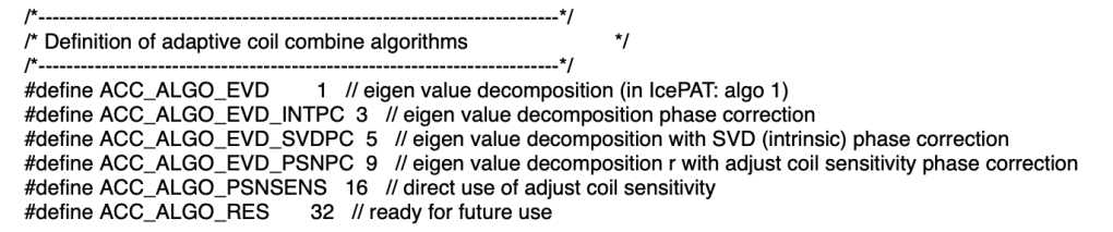
If you want to reconstruct the same data with different coil combination algorithms retrospectively, you can do so my means of TWIX:

YAPS.AdaptiveCoilCombineAlgo. The default of -1 gives ACC_ALGO_EVD_PSNPC = 9 which uses the body coil reference (PSNPC = Pre Scan Normalize – i.e. use at 3T). Instead, you can set ACC_ALGO_EVD_SVDPC = 5 which uses the virtual reference coil (i.e. use at 7T). (note: this seems to not work with “meas dependencies” on!). The name of this implementation is: Singular Valued Decomposition Phase Combination.

Note that very old VB15/VB17 adaptive combine coil-combination methods were not optimized for fMRI. Those algorithms estimated the coil-weights for every TR separately. This is not longer a problem for VE scanners.

Acknowledgements: I want to thank Rüdiger Stirnberg and Simon Robinson for explaining the above to me.

42) How to cite?

When you are publicly presenting results that have been acquired with this sequence, it would be great if you could cite us. E.g. you could include the snippets:

We used a 3D-EPI sequence (Stirnberg and Stöcker 2021) with VASO preparation (Huber et al., 2021) (version [insert your version hash here. E.g. 822d59f4]).

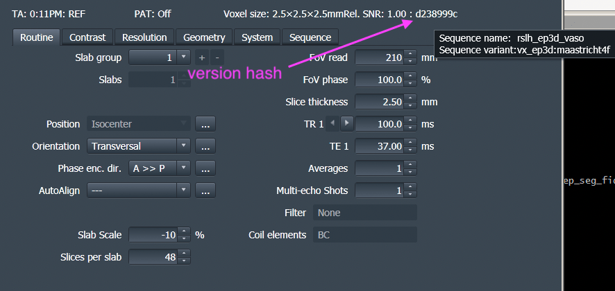
44) Which sequence version do I have?

You can find out which version you are using in the protocol editor (aka DotCockpit). The version hash is displayed on the top right. If you hoover over it with the mouse, you see the sequence name too.

Version history:

version hash	AKA		characteristic or new
822d59f4	GLAS dd309e05 (DZNE)		with segmentation factor
dd309e95			same as 822d59f4 but for VE11E
a8839449	maastricht4d	modify Icepat MOSAIC MAGN per shot	EXT TI-fix with MAGEC7 OccationalPerTR-fix
822d59f4	maastricht4a		EXT TI-fix
5361868e	maastricht4a		EXT TI-fix
0c0b7b73c 0c0b7b7	maastricht4a		with and without TI bug
253c3470 (DZNE)	dzne_irep3d
684e6dda	maastricht4e	modify Icepat MOSAIC MAGN per shot	NORDIC noise scanns
d238999c	maastricht4f	Compiled for VE12U_SP01 on 20210721	with NORDIC and Phiilip’s new recons stuff
26dc5a59	maastricht4j	all supported platforms	New functor Name, symmetric TI, alternating RO, single NORDIC pair

45) I want to change the protocol to set GRAPPA in y-direction to zero, but the protocol editor wouldn’t let me do it.

If you want to switch between GRAPPA in one direction and/or use a larger segmentation factor instead, it can matter on the order what you change first.

E.g. first temporarily increase the GRAPPA factor in the z direction. Then the protocol editor should allow you to lower the GRAPPA factor in the y-direction. Afterwards, you can then switch off the GRAPPA factor in the z direction again, if you want.

46) What is the standard way of making the data of this sequence BIDS compatible?

Remi Gau kindly provided a template of BIDS compatible VASO data in this repository: https://gin.g-node.org/RemiGau/ds003216/src/bids_demo.

Any sequence version that is provided after June 2022, contains an updated MOSAIC functor that sorts imaged with different inversion times in separate time series. This allows users to BIDS-ify the separate time series with the extensions of _cbv and _bold, according to the BIDS standard.

The image time series are written out in the order they are acquired in. This means that the blood-nulled (VASO). time series are written before the non-nulled (BOLD) time series.

Acknowledgement of contributions to the reconstruction

Parts of the recommended mosaic reconstruction code comes with the courtesy of Ben Poser and Philipp Ehses. The interface to optimize IcePat with respect to GRAPPA Kernel size and regularization is kindly provided by Philipp Ehses. We also want to thank Denis Chaimow for valuable feedback regarding a temporary bug of the units of the inversion delays of previous sequence versions.

Further background information: Lecture about the benefits or 3D-EPI readouts for fMRI

Educational lecture section from Renzo comparing 3D-EPI to SMS (MB) and its respective benefits.

Educational lecture section from Rüdi about the differences of 3D-EPI to SMS (MB) and its respective benefits.

References

• [Poser2010] Poser, B. A., Koopmans, P. J., Witzel, T., Wald, L. L., & Barth, M. (2010). Three dimensional echoplanar imaging at 7 Tesla. NeuroImage, 51(1), 261–266.
• [Stirnberg2021] Stirnberg R., Stöcker, T. (2021). Segmented K-Space Blipped-Controlled Aliasing in Parallel Imaging for High Spatiotemporal Resolution EPI. Magnetic Resonance in Medicine.
• [Stirnberg2019] Stirnberg, R., Dong, Y., Bause, J., Ehses, P., & Stöcker, T. (2019). T1 Mapping at 7T Using a Novel Inversion-Recovery Look-Locker 3D-EPI Sequence. In Proceedings of the International Society of Magnetic Resonance in Medicine.
• [Huber2021] Huber, L., Finn, E. S., Chai, Y., Goebel, R., Stirnberg, R., Stöcker, T., Marrett, S., Uludag, K., Kim, S. G., Han, S., Bandettini, P. A., & Poser, B. A. (2021). Layer-dependent functional connectivity methods. Progress in Neurobiology, 101835. https://doi.org/10.1016/j.pneurobio.2020.101835
• [Stirnberg2017] Stirnberg, R., Huijbers, W., Brenner, D., Poser, B. A., Breteler, M., & Stöcker, T. (2017). Rapid whole-brain resting-state fMRI at 3 Tesla: Efficiency-optimized three-dimensional EPI versus repetition time matched simultaneous-multi-slice EPI. NeuroImage, 163(August), 81-92.
• [Stirnberg2018] Stirnberg, R., Deistung, A., Reichenbach, J., & Stöcker, T. (2018). Accelerated quantitative susceptibility and R2* mapping with flexible k-t-segmented 3D-EPI. In Proceedings of the International Society of Magnetic Resonance in Medicine.
• [Stirnberg2016] Stirnberg, R., Brenner, D., Stöcker, T., & Shah, N. J. (2016). Rapid fat suppression for three dimensional echo planar imaging with minimized specific absorption rate. Magnetic Resonance in Medicine, 76(5), 1517-1523.