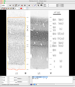
Often we would like to normalize depth-dependent fMRI signals and assign it to specific cytoarchitectonially defined cortical layers. However, we often only have access to cytoarchitectonial histology data in the form to figures in papers. But since we only have the web-view or the PDF available, we cannot easily extract those data as a layer-profile. Since most layering tools are designed for nii data only, paper figures (e.g. jpg or GNP) are not straight-forwardly transformed to layer profiles.
In this blob post, I describe a set of steps on how to convert any paper figure into a nii-file that allows the extraction of layer profiles.
Introduction
Most layering tools are designed to work in 3D-space of nii images. But paper figures mostly only be accessed as pdfs or screenshot PNGs. Thus, the major challenge to obtain layer profiles of paper figures is to convert PNG to nii. Here, I describe the preparation of the png to make it convertible to nii. And then I will describe how to do the nii-header manipulation to make it readable for layering tools.
The following steps are necessary:
- taking screen shot
- convert PNG to a usable datatype (e.g. with GIMP)
- converting PNG to NII (e.g. with MIPAV)
- generating a consistent header (e.g. with fsledithd)
- generating layers in NII (e.g with LN_GROW_LAYERS)
- extracting profiles (e.g. with afni)
1.) Taking a screenshot
Taking a screenshot n you laptop is straightforward. E.g. on mac its the key-short-cut “command+shift+4”.

2.) converting PNG to usable datatype
In a layer profile, we are interested to only plot one dimension (one y-axis). E.g. a gray-value. Even-though, the nii-standard supports datatype 124 (RGB), most nii-viewers and nii-tools do not work with it. Hence, we need to convert the PNG-figure into a datatype 4 figure. I find GIMP useful for doing this.

3.) converting PNG to NII
Fortunately, the program MIPAV can convert PNGs to nii relatively straight forwardly.
After you started MIPAV, you can open any image in “File”->”open image from file”. And then you can save it as “nii”.
This step generates the a nii file.
4.) generating a consistent header
Since the nii file is only converted from a 2D-picture, the nii-header suggests its a 2D image too. However, since most nii-tools (e.g. FSL, afni, LAYNII) work in 3D-space, they cannot read this nii-file, unless we make it a 3D-file.
The header can be easily fixed with the FSL tool fsledithd.

This step generates a nii file that can be read in afni, and LAYNII.
5.) generating layers in NII
Now that the figure is in nii format, the layering can be done as in any other nii-dataset. I described how to do this in more detailed fashion in this blog post:
In short, I use FSLview to draw at the borderline between GM and CSF as “1” and the borderline between GM and WM as “3”. Then I fill everything with “3” that is GM and save it as “rim.nii. Fianlly, I run “LN_GROW_LAYERS -rim rim.nii”, which generates a nii-files with 21 layer masks.
6.) extracting profiles
With the generated layer mask, its just a matter of averaging the signal in the respective layers. This is described here using 3dROIstats. In short: I use this script to extract the average layer values into a text file and then I use this gnuplot script to plot it.


