Authors: Lasse Knudsen, Luca Vizioli, Federico De Martino, Lonike Faes, Dan Handwerker, Renzo Huber
This post describes the usage, capabilities and challenges of NORDIC PCA denoising on VASO data. A video presentation of this project can be found here: https://youtu.be/bbGKMTWVrJY.
Are you ever annoyed how hard it is to get brain data off the scanner? The fact that scanners usually contain private information about patients and are thus embedded in maximally restrictive clinical cyber-security environments, makes it quite complicated to get access to the data. Especially when visiting collaborative sites.
In this this Hackathon project, we aim to develop a purely uni-directional (safe) data streaming “hack” to transfer MRI data directly to the cloud by means dynamic QR codes.
In the early days of the Internet, modems (modulator-demodulator) were used to (i) convert digital information into audio streams, (ii) transfer them across telephone lines, and (iii) convert them back into the digital domain. Here, we aim to do the same thing with pixel data of MRI scans. However, instead of audio signal we will use machine-readable visual information: QR codes.
Specific aims of the Brain QR modem
1.) We will develop an ICE-Functor that converts pixel data to QR codes in real time
2.) We will develop an Android app that converts the streamed QR coded into a series of png that are directly streamed to the cloud (Drive folder).
3.) We will develop a LayNii program that converts stacks of PNG images into Nii files.
This project contains many consecutive components of a modem. And will likely take 2-3 rounds of Hackathons to be completed.
The purpose of this blog post is to provide guidance on how to get started with the layer-fMRI analysis suite: LAYNII. This post is an extended version of the LAYNII README.
When you want to analyze functional magnetic resonance imaging (fMRI) signals across cortical depths, you need to know which voxel overlaps with which cortical depth. The relative cortical depth of each voxel is calculated based on the geometry of the proximal cortical gray matter boundaries. One of these boundaries is the inner gray matter boundary which often faces the white matter and the other boundary is the outer gray matter boundary which often faces the cerebrospinal fluid. Once the cortical depth of each voxel is calculated based on the cortical gray matter geometry, corresponding layers can be assigned to cortical depths based on several principles.
One of the fundamental principles used for “assigning layers to cortical depths” (aka layering, layerification) is the equi-volume principle. This layering principle was proposed by Bok in 1929, where he tries to subdivide the cortex across little layer-chunks that have the same volume. I.e. gyri and sulci will exhibit any given layer at a different cortical depth, dependent on the cortical folding and volume sizes (see figure below).
With respect to applying equi-volume principle in layer-fMRI, the equi-volume layering has gone through quite a story. A plot with many parallels to Anakin Skywalker.
In this blog, the equi-volume layering approach is evaluated. Furthermore, it is demonstrated how to use it in LAYNII software.
How can one assign layers to discrete voxels? Is it possible to perform topographical fMRI analyses across layers and columns directly in the original voxel space that raw data from the scanner come in?
The MP2RAGE sequence is very popular for 7T anatomical imaging and is very commonly used to acquire 0.7-1 mm resolution whole brain anatomical reference data. Aside of this common application, it can also be very helpful for layer-fMRI studies to obtain even higher resolution T1 maps in the range of 0.5mm iso. However, when optimizing MP2RAGE sequence parameters for layer-fMRI studies, there are a few things that might be helpful to keep in mind.
In this post, I would like to discuss the challenges of using the popular MP2RAGE sequence in layer-fMRI studies. Specifically I will discuss challenges/features regarding:
In this blog post I want to go through the analysis pipeline of layer-dependent VASO.
I will go through the all the analysis steps that need to be done to go from raw data from the scanner to final layer profiles. The entire thing will take about 30 min (10 min analysis and 20 min explaining and browsing through data).
During the entire analysis pipeline I am using the following software packages: SPM, AFNI, and LAYNII, and gnuplot (if you want fancier plotting tools)
In this blog post, I want to share my thoughts on the number of layers that should be extracted from any given dataset. I will try to give an overview of how many layers are usually extracted in the field, I’ll describe my personal choices of layer numbers, and I will try to discuss the challenges of layer signal extraction along the way.
In this blog post Sri Kashyap and I describe how to deal with the registration of high-resolution datasets across days, across different resolutions, and across different sequences.
I am particularly fond of the following two tools: Firstly, ITK-SNAP for visually-guided manual alignment and secondly, using ANTs programs: antsRegistration and antsApplyTransforms.
Maximum intensity projection and minimum intensity projection can be insightful for mapping of vessels in 3D-slabs. In this post, I describe the application of intensity projections with LAYNII.
CBV-fMRI with VASO is highly dependent on a good inversion contrast. It gives it its CBV sensitivity and is also responsible for most of the VASO specific pitfalls (e.g. inflow, CSF etc. ). And thus, it should be optimized as much as possible.
In this blog post, I want to describe the most important features of a reliable inversion pulse for the application of VASO at 7T with a head transmit coil.
ISIS-conv is a very useful dicom to nii converter from Enrico Reimer. ISIS-conv gets along with a lot of challenging data sets that no other converter (that I know of) can handle so conveniently:
SMS-data, where individual slices have a non-constant inter-slice distances.
VASO data with non-constant TRs
Multi-echo, multi-coil, and Magnitude/Phase data.
There is a Mac-installation package of ISIS-conv. Unfortunately, however, with every IOS update, it has become more complicated to install it.
Since, I spend too much time figuring out how to install it after every update, I am collecting the necessary steps in this Blog post for future reference:
In this blog post, I want to write about pipelines on how to prepare Nifti-brain data and make them printable by a 3D-printer.
Two pipelines are shown. One pipeline describes the 3D-printing the cortical folding structure that is estimated with Freesurfer and subsequently corrected with Meshlab. And another pipeline describes how you can 3D-print any binary nii-volume by using the AFNI-program IsoSurface and correct the output with netfabb. Continue reading “3D-printing nii data”→
Often we would like to normalize depth-dependent fMRI signals and assign it to specific cytoarchitectonially defined cortical layers. However, we often only have access to cytoarchitectonial histology data in the form to figures in papers. But since we only have the web-view or the PDF available, we cannot easily extract those data as a layer-profile. Since most layering tools are designed for nii data only, paper figures (e.g. jpg or GNP) are not straight-forwardly transformed to layer profiles.
In this blob post, I describe a set of steps on how to convert any paper figure into a nii-file that allows the extraction of layer profiles.
In layer-fMRI, we spend so much time and effort to achieve high spatial resolutions and small voxel sizes during the acquisition. However, during the evaluation pipeline much of this spatial resolution can be lost during multiple resampling steps.
In this post, I want to discuss sources of signal blurring during spatial resampling steps and potential strategies to account for them.
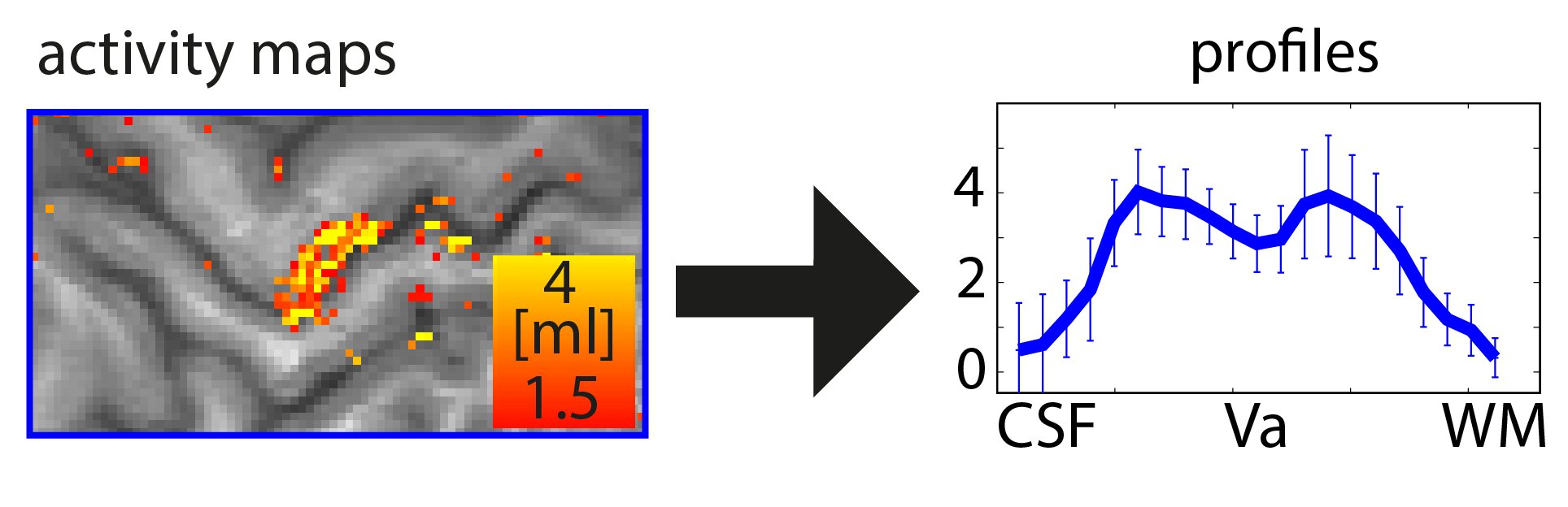
This is a step-by-step description on how to obtain layer profiles from any high-resolution fMRI dataset. It is based on manual delineated ROIs and does not require the tricky analysis steps including distortion correction, registration to whole brain “anatomical” datasets, or automatic tissue type segmentation. Hence this is a very quick way for a first glance of the freshly acquired data.
This post shows how you can get from activation maps to layer-profiles in 10 min. In a quick and dirty way.
The important steps are: 1.) Upscaling, 2.) Manual delineation of GM, 3.) Calculation of cortical depths in ROI, 4.) Extracting functional data based on calculated cortical depths.